Analogy

Let’s pretend that you’re a meteorologist. One of your roles as a meteorologist is to forecast the weather. The people in your area rely on your weather predictions being accurate. They check the weather forecast to know what to wear for the day, optimize travel plans, and prepare in case they need extra gear (i.e., umbrella, sunscreen, etc.). That is to say – you want your weather predictions to be as accurate as possible, such that the discrepancy between the actual weather and the weather you predicted is minimized. There are different methods that can be used to accurately predict the weather based on information we already have. One of those methods is ordinary least squares (OLS) estimation.

Diagram

In the case of predicting the day’s temperature …

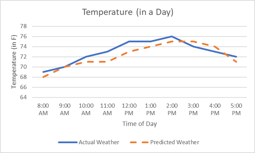
The above figure is a representation of the preferred outcome (given that you won’t be 100% accurate all the time). After you predicted the weather for each of the recorded timepoints, it was plotted and compared to the actual weather. In this diagram, you were off by two degrees Fahrenheit, at the most. Thanks to you, the locals were able to go out in comfortable clothing without getting too hot or too cold.

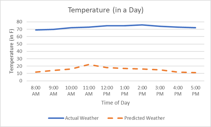
This diagram represents a worse scenario. The actual weather was set to be low- to mid- 70’s – but you predicted it to be in the ‘teens and 20’s. In this scenario, the locals are outraged (and suffering mild heatstroke) after going out in winter parkas and winter gear, only to be met with temperate weather.

In these diagrams, you’re shown the importance of estimating the temperature so that the difference between the actual and predicted weather is minimal. We know our predictions won’t be perfect. Ideally, the over- and under-estimations of the temperature would average out to (close to) zero. In addition to this, we want the differences between actual and predicted temperature is minimal.

Example

As an example, pretend we have a dataset containing data for the number of hours students spent studying for an exam and their scores on the exam. We want to produce a model that can be used to predict exam scores from hours spent studying.

Ordinary Least Squares estimation could be used to estimate the intercept and slope values that minimize the difference between the observed Exam Scores and the predicted Exam Scores – or minimize the squared residuals. This is preferred over estimating values that do NOT minimize the residuals, or differences between the predicted and observed values.

Plain Language Definition

Ordinary Least Squares estimation is a method used to estimate the “best-fitting” line through a set of observed data points. This “line of best fit” is created in a way that minimizes the total difference between the observed and predicted outcome variable values. This is so the line can best represent the relationship between the variables in the data.

Technical Definition

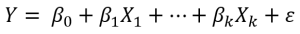
Ordinary Least Squares (OLS) estimation is a method used to estimate the parameters in a regression model to minimize the sum of squared errors (SSE; ). This method creates a line through the data points that minimizes the squared residual between the observed values of the outcome variable and the corresponding predicted values of the outcome variable.

OLS estimation comes with a number of assumptions. These include:

• Model is linear in parameters and correctly specified
  • o This assumption addresses the functional form of the model

• o The β’s are the parameters that OLS estimates

• Random sample of n observations
  • o If the data are random, the residuals are statistically independent/uncorrelated with each other
• Mean of the residuals has an expected value of zero
  • o The residual, or error term, accounts for the variation in the outcome variable that the predictor variable(s) do not explain
  • o For the model to be unbiased, the average value of the residuals should be equal to zero
• Homoscedasticity of residuals
  • o The variance of the error term should be consistent across the range of the predictor variable(s)
  • o Heteroscedasticity (varying variance) reduces the precision of the estimates
• Residuals are normally distributed
  • o Satisfying this assumption allows statistical hypothesis testing to be done and reliable confidence intervals to be generated
• No measurement error in the predictor variables
  • o Measurement error in the predictor variables leads to biased unstandardized regression weights (b)

Violation of OLS assumptions tend to impact:

• Unbiasedness
  • o Parameter estimates will be biased (incorrect)
• Efficiency
  • o Standard error estimates will be incorrect – inefficient