Fluorescent molecules (fluorophores) are typically described by their spectra—the ranges of wavelengths at which they are excited and at which they emit. Knowing a fluorophore’s characteristic spectra allows one to selectively visualize the molecule, distinguishing it from non-fluorescent objects and fluorescent objects with different excitation and/or emission spectra. This selectivity is based on intensity: only fluorescent objects with spectra that match the excitation and emission wavelengths used will appear bright in the image and all other objects will appear dark. However, fluorescent molecules have another characteristic that enables their identification and is not based on intensity: their fluorescence lifetime (hereafter simply called “lifetime”). Lifetime can be used to differentiate a fluorophore from other types of fluorophores and background fluorescence even in cases where they all have similar spectra. In special situations, lifetime can also be used to indicate something about a fluorophore’s local environment and thereby serve as molecular sensor.

Fluorescence Lifetime

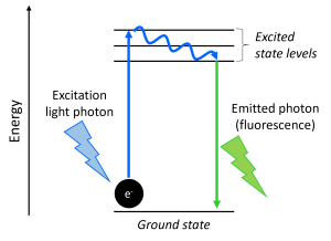
Fluorescence lifetime is the delay between when a fluorophore is excited and when it emits light. For the purpose of this explanation, it is easier to think about light in terms of particles or individual units called photons. Fluorescence occurs when a photon of excitation light excites an electron (e-) in the fluorophore and then, a short time later, the electron relaxes back to its ground energy state and releases energy as a photon (fluorescence emission) (Fig. 1). The “short time” between when the photon excites the electron and the relaxing electron produces a photon of fluorescence is the molecule’s fluorescence lifetime. Note that the lifetime is not the amount of time that the molecule emits light (one photon is produced and it travels at the speed of light) but the delay between the excitation and emission. Because typical lifetimes are on the order of nanoseconds, we do not notice the delay. Different types of fluorescent molecules have different lifetimes and a molecule’s lifetime can be affected by its environment (e.g. pH, polarity). It is also important to note that, since this is a physical process, there is a certain amount of random variability and a fluorophore’s lifetime will vary slightly over multiple excitation/emission events. When a fluorophore’s characteristic lifetime is reported, this is its “average” lifetime.

Fluorescence Lifetime Measurements

In fluorescence lifetime imaging microscopy (FLIM), as in normal fluorescence microscopy, you excite your fluorophores and collect their emission using the optimal wavelengths defined by their spectra. You also still collect intensity information and can see an image based on fluorescence intensities (i.e. a “normal” fluorescence image). However, when the microscope is operated in FLIM mode, it will also simultaneously collect lifetime information. It does this basically by exciting the sample, starting a super-precise stopwatch, and then recording the times when the photons arrive at the detector. Because the microscope needs to wait after the sample is excited to allow time for the resulting emitted photons to be collected and timed, the specimen cannot be illuminated continuously. Instead, the specimen is illuminated in short bursts (pulses) spaced sufficiently far apart in time to allow for the emitted photon collection. Because fluorescence lifetimes are so short, the pulses can occur so quickly that you will not notice them; the laser will appear to be firing continuously.

The Stellaris performs this measurement pixel-by-pixel. Because there are likely many (100s, 1000s?) fluorophores within the volume corresponding to a single pixel, the detector will collect many photons over many excitation pulses. The photons will not all arrive at the same time (remember there is random variability); instead, there will be a distribution of lifetimes from which the system can calculate an “average” lifetime. Using this information, the microscope can then display an image in which the colors correspond to lifetime instead of intensity. The Stellaris has two different methods for analyzing the lifetime data and calculating “average” lifetimes: TauSense and FALCON.

TauSense uses a fast, semi-quantitative approach that is best-suited for separating different fluorescent components based on lifetime. It essentially calculates a simple average of the lifetimes of the photons collected at each pixel. It is useful for identifying and separating autofluorescence (intrinsic fluorescence coming from natural compounds in your specimen) from the real fluorescent signal you are trying to visualize. This method can also be used to distinguish between two fluorophores with similar spectra but different lifetimes. The lifetime values produced by this method should only be treated as rough estimates. If your research question depends on having precise lifetime values, you should use FALCON.

FALCON uses a slower, quantitative approach that involves post-acquisition analysis steps and is best-suited for rigorous analyses of complex mixtures of, or changes to, fluorescence lifetime. Rather than calculate a simple average, this method generates a histogram of all lifetimes recorded within a pixel and then fits the data to a mathematical model to calculate a single lifetime value that characterizes the fluorophore. This is the rigorous way to calculate lifetime and produces values that can be compared to published lifetimes. Use this method for analyses that require precise lifetime calculations such as fluorescence resonance energy transfer (FRET) and FLIM-based biosensors. Because this method uses curve fitting, it is especially suited for situations where there are multiple distributions of fluorescence lifetimes in the sample.

If you use either type of FLIM, you will need to report addition parameters in your methods beyond those for standard confocal microscopy (see the Data Management chapter). For TauSense applications, you should specify the cut-off lifetimes used to separate different populations. For FALCON, you will need to report multiple aspects of your analysis—talk with Dr. Kubow. Because there are so many parameters associated with FLIM, it is good practice to make the raw and processed images publicly available so that others can compare them and access the images’ full metadata.