Fluorescence microscopy is a very powerful way to visualize difficult-to-see objects, in particular because fluorescent probes can be designed to recognize objects with high specificity. The design of fluorescent probes is beyond the scope of this short reading. Suffice it to say that, in fluorescent microscopy, specimens are labeled (stained) with fluorescent dyes (also known as fluorophores) that emit light that can be seen using a microscope.

Physical Basis of Fluorescence

First, it is important to remember the correspondence between the wavelength of light and color (Fig. 1) and that wavelength and energy are inversely related. For example, ultraviolet light (can cause sunburn) is higher energy than infrared light (used, e.g., in some remote controls and thermometers).

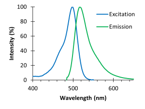
Fluorescence is a property of some atoms and molecules to absorb light and, after a brief interval, to re-emit light. Each type of fluorescent molecule can absorb light only of specific wavelengths, and also only emits light of specific wavelengths. These are represented graphically as excitation and emission spectra, where the peaks indicate the wavelengths that best excite the molecule and are most frequently emitted, respectively. Figure 2 shows the spectra for fluorescein, which was one of the first synthetic fluorescent dyes. Fluorescein is excited best by ~490 nm light, but can also be excited (although not as well) by other wavelengths from 400-530 nm. When excited, fluorescein will most often emit ~510 nm light, but might also emit light with wavelengths from 490-640 nm, although not as often. The wavelength of the emitted light is always greater than the wavelength of the excitation light because there is energy loss in this process and wavelength and energy are inversely related.

Different fluorescent molecules have different characteristic excitation and emission spectra and are colloquially referred to by the color of their peak emission light (not their excitation light). Fluorescein is considered a “green” dye because it emits green light. Fluorophores are often grouped together by their emission wavelengths. For example, Alexa 488 and Green Fluorescent Protein are also considered “green” dyes: although their spectra are different, they all emit green light.

Fluorescence Microscopy

Fluorescence microscopes contain glass filters that only transmit specific wavelengths of light. These filters are used to select the wavelengths necessary to excite a fluorophore and capture its emission. The light path of a fluorescence microscope is different than that of a transmitted light microscope:

1. White light (containing a broad range of wavelengths) enters the microscope and encounters the excitation filter. Only wavelengths necessary to excite the fluorophore pass through the filter; all others are blocked. For example, the excitation filter for a green dye might pass 450-490 nm light.
2. The excitation light is directed by a special mirror (“dichroic” mirror) so that it emits out of the objective and illuminates the specimen. This is a major difference from a transmitted light technique where the light emits from the condenser.
3. The fluorophores in the specimen are excited and emit light at a longer wavelength.
4. The emitted light is collected by the objective and is directed by the dichroic mirror toward the emission filter. Only wavelengths emitted by the fluorophore are allowed to pass; all others are blocked. For example, the emission filter for a green dye might pass 500-550 nm light. The emission filter might seem unnecessary, but consider that the objective is not only “seeing” the specimen’s fluorescence, but also the excitation light. The emission filter blocks the excitation light and ensures that the specimen is completely dark except for the areas labeled by the fluorophore.
5. The light then travels to the oculars and/or camera.

Note that different microscopes may use slight variations of this strategy. For example, some microscopes use high-intensity LEDs with narrow wavelength ranges instead of a white-light source.

Excitation and emission filters are paired in filter sets (or “filter cubes”), each designed to image one family of fluorophores (one set for green, one for red, etc.). Filter sets are often named by the name of the fluorophore for which they were designed (e.g. “Fluorescein”). Realize, however, that the set works for any fluorophore that can be excited and emits in the ranges dictated by the set’s filters (e.g. a “Fluorescein” set would also all you to image Alexa 488 and Green Fluorescent Protein).

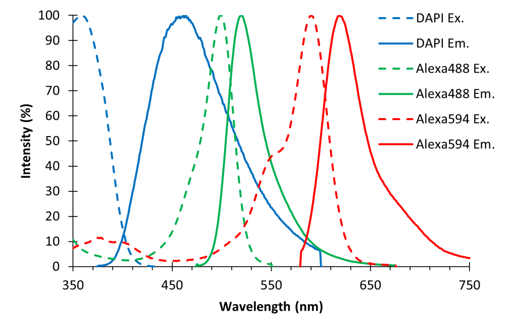
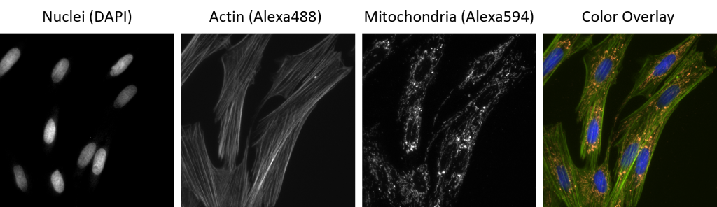
It is possible to label and image different features of a specimen simultaneously using different “colors” of fluorophores. For example, you could label nuclei with DAPI (a blue dye), actin with Alexa 488 (a green dye), and mitochondria with Alexa 594 (a red dye). You can visualize each of these fluorophores independently by changing filter sets (Fig. 3). During your training, you will learn how to determine which filter set is correct for your fluorophore(s).

Since you are only ever looking at one “color” of fluorophore at a time, there is no need to use a color camera. Most fluorescence microscopes are equipped with monochrome (“black and white”) cameras because they are more sensitive than color cameras. In the earlier example, you would acquire a monochrome image using each of the three filter sets and these three images would then be colored and combined using a computer program (Fig. 4). Remember from the Digital Imaging chapter that monochrome images can be displayed in whatever color your desire.

Photobleaching

One major problem with fluorescence microscopy is photobleaching. Fluorescent molecules can only be excited a finite number of times before they become damaged and no longer fluoresce. The phenomenon of fluorophores “dying” or “going dark” is called photobleaching. The practical implication of this is that the longer you shine excitation light on your specimen, the more fluorophores you will “kill” and the dimmer your specimen will become until you can no longer see any fluorescence emission. To minimize photobleaching, only illuminate your sample when you are actively viewing or imaging your specimen.

Image Intensity Scaling Adjustments

Fluorescent stains are often dim and require higher illumination (excitation) light intensity and camera exposure times than brightfield imaging. Even so, sometimes it is impossible to obtain a bright fluorescence image. In such cases, we can adjust the image intensity scaling to allow us to see the fluorescent signal. In most imaging software, this scaling is accomplished using an interface displaying the histogram of all the intensities in the image. The image histogram x-axis is intensity and the y-axis (usually shown on a log scale) is the number of pixels (“count”). Fig. 5A shows a very dim image and its histogram. The bars of the histogram are all close to the zero-end of the x-axis illustrating, indicating that all the pixels in the image have very low intensities corresponding to shades of gray nearly indistinguishable from black.

We can make the image brighter by decreasing the upper scaling limit (Fig. 5B), which in most imaging software is done by dragging a vertical line at the right side of the plot to the left (illustrated as a red line in the figure). Doing this tells the computer to display every pixel with a value higher than the upper limit (30 in this example) as white and then redistribute all the shades of gray over the lower-value pixels. This is illustrated by the grayscale “bar” underneath the histogram.

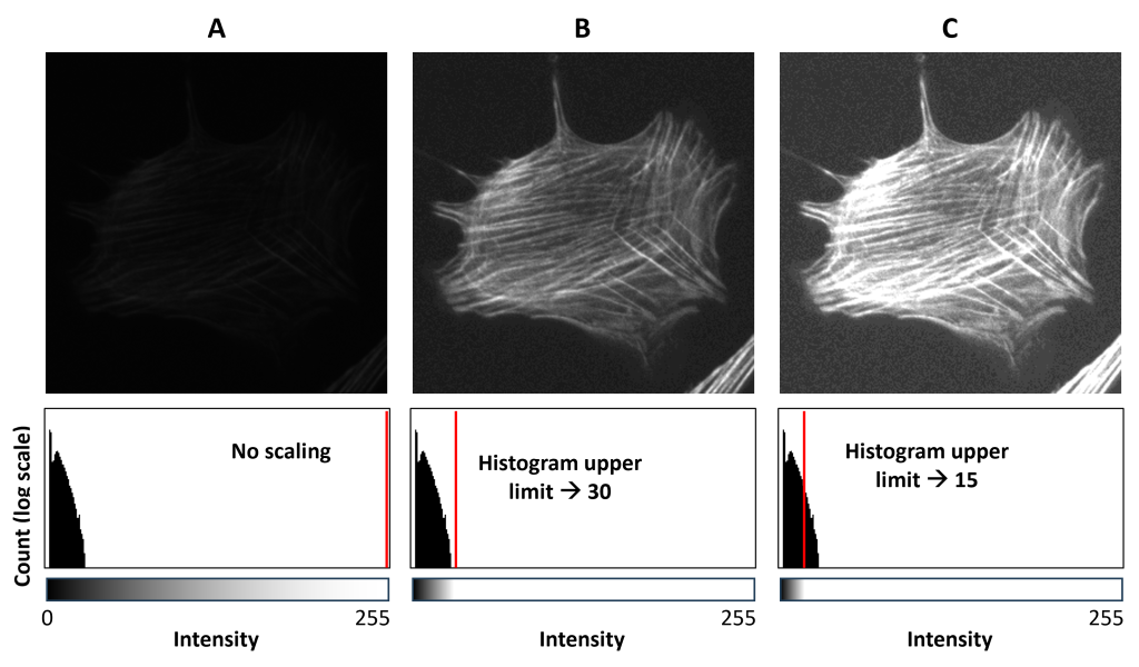
You can, of course, go too far and make the image too bright. Fig. 5C has the upper limit set even lower and illustrates that all pixels above the limit will be displayed as white regardless of their relative differences in intensity. This panel also shows that, if you move the upper limit too far to the left, you may start to see the background noise of the camera (note the “fuzzy” background relative to the other panels).

Note that doing this does not actually change the image data. It doesn’t make the image brighter by changing the pixel values–it makes the image appear brighter by changing how the computer displays it. Therefore, this is not a substitute for acquiring good images in the first place.