3 Chapter 3: Simulation Basics – How a System Dynamics Simulation Model Works

3.1. Why Build a Running Simulation Model?

You are now well on your way to working like a systems thinker! You’ve learned about the importance of seeing problems in terms of their behavior over time, instead of focusing merely on isolated events. You’ve learned how to describe the system behind that behavior by looking for feedback loops, stocks, and flows. You’ve learned how to describe the roles of these components by using causal loop diagrams (CLDs) or stock and flow diagrams (SFDs).

But now what? How can we use these ideas and tools to help us make better decisions? One of the best ways to do this is to create a running simulation model of a problem and see how your hypothesized system structure affects behavior over time. To do this, we convert our SFD into a computer model.

Using a carefully constructed system dynamics computer simulation model can be a game-changer for a decision maker.  Back in 1907, the decision makers working on the Kaibab Plateau did not have the ability to “experiment” on a computer. Instead, they experimented on the real-life ecosystem. Because of all the feedback dynamics, stocks, flows, and delays in this system, the results of their efforts took years to play out — and they were disastrous! The deer population exploded (“irrupted” in ecological terms), and the deer over-grazed the forest on the plateau, leading to a near-collapse of the entire ecosystem!  Ecologists have been working on this problem ever since!

We shouldn’t be too critical of those early decision makers. They didn’t have access to a methodology like system dynamics, nor did they have ready access to computers that we enjoy today. In addition, feedback-rich systems like the Kaibab ecosystem are notoriously difficult to understand or manage “on the fly.” This shouldn’t surprise you.  You had a similar experience when you were asked to make decisions using only the same information that was available to decision makers back then.

But what if those decision makers had access to a computer simulator where they could learn how the system might respond to their actions, try out different policies for managing the balance between the predators, livestock, deer, and forest, and explore the long-term consequences of their actions before doing anything with the real-life system?

That’s where this chapter comes in. You will learn some of the basics of building running models of problems like the Kaibab, and you will get a chance to validate your simulator against real data. You will then learn how to use the model to explore options for managing the resources on the Kaibab in a sustainable way.

But building a simulator is somewhat like building a car engine. To build a car engine, you’d need to know some basics about the parts of the engine and how they work together to move a car down the road. You have to “peek under the hood” of a car and see the main parts of the motor, how they fit together, and how they work. In the same way, if you want to build a system dynamics model, you have to “peek under the hood” and learn how one of these models works. We’ll do this by examining a simple model involving stock and two flows with some balancing and reinforcing feedback.

3.2. Simulation Basics: The Net Flow and its Effect on a Stock

In Figure 6 we used a bathtub with a faucet and drain to explain the relationship between a stock and its flows. This analogy can be further used to illustrate how the contents of a stock are affected by its attendant flows. Understanding how this works provides us with just the “peek under the hood” that we need in order to start building a simulation model.

First, common sense tells us that if the faucet adds water faster than the drain removes it, the bathtub will accumulate water; its water level will increase. Of course, if the drain is so large that the faucet doesn’t add water as fast as it drains out, the water level in the tub will drop. This is true no matter how many faucets or drains you have! As long as the total inflow of water exceeds the total outflow, the water level in the tub will increase. If the total inflow is less than the outflow, the water level in the tub will drop.

Another way of saying this is to refer to something called the net flow into the tub. At any moment in time, the net flow into a stock refers to the total of all the inflows minus the total of all the outflows connected to that stock. If the net flow is positive, then more water is coming in than is going out, and the water level in the tub will increase. If the net flow is negative, more water is flowing out than is coming in; the water level in the tub will drop.  We can summarize all of this as follows.

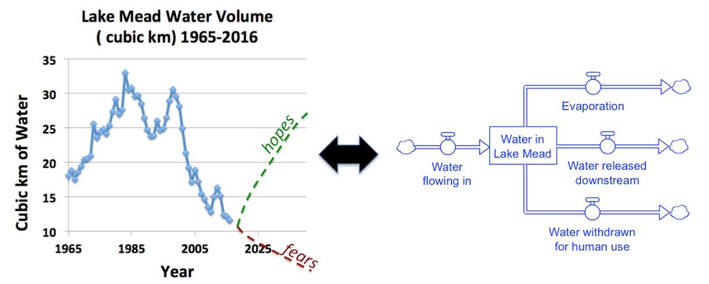
In order to illustrate these ideas with a concrete example, consider the amount of water in a lake. This quantity of water can be represented as a stock with flows running into and out of it.  Figure 11 shows a BOTG of the water volume in Lake Mead, Nevada, as measured at midnight on August 2 every year.  Lake Mead is of particular interest because it provides water for millions of people in Arizona, California, and Nevada and for large agricultural activities in the region.  The solid line shows historic water volume in Lake Mead from 1965 through 2016. The two dashed lines show our hopes and fears for the future.  To the right of the graph is a stock and flow diagram that identifies the stock (i.e, the Water in the Lake) and several flows that affect the water level.  It is clear from Figure 11 that the Lake Mead water levels have varied dramatically over the past several decades.  It’s also clear that water levels have overall declined for the past 2 decades.

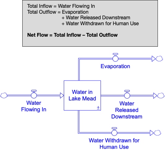
But what causes the variation in Lake Mead water level? A host of factors contribute to this, including interactions between population growth, fluctuating weather patterns, and land use in the region. However, the bathtub analogy in Figure 6 tells us that the only way Lake Mead water levels can change is through the flows that are connected to the Lake Mead stock.  For example, Figure 11 shows four flows affecting the water in Lake Mead. While there are likely other flows that should be considered, we’ll restrict ourselves to these four to keep this illustration relatively simple. The important thing to remember is that whatever flows are connected to the stock, the effects of population, weather, land use, and other factors on Lake Mead’s water levels come about only as population, weather, etc. impact the rates of the flows running into and out of the lake.

Assuming the simplified flow structure in Figure 11, we can explore how the net flow into Lake Mead impacts the water level.  Recall that the net flow is calculated as the total of all the inflows minus the total of all the outflows. Using Figure 12, we see that the net flow is calculated as follows.

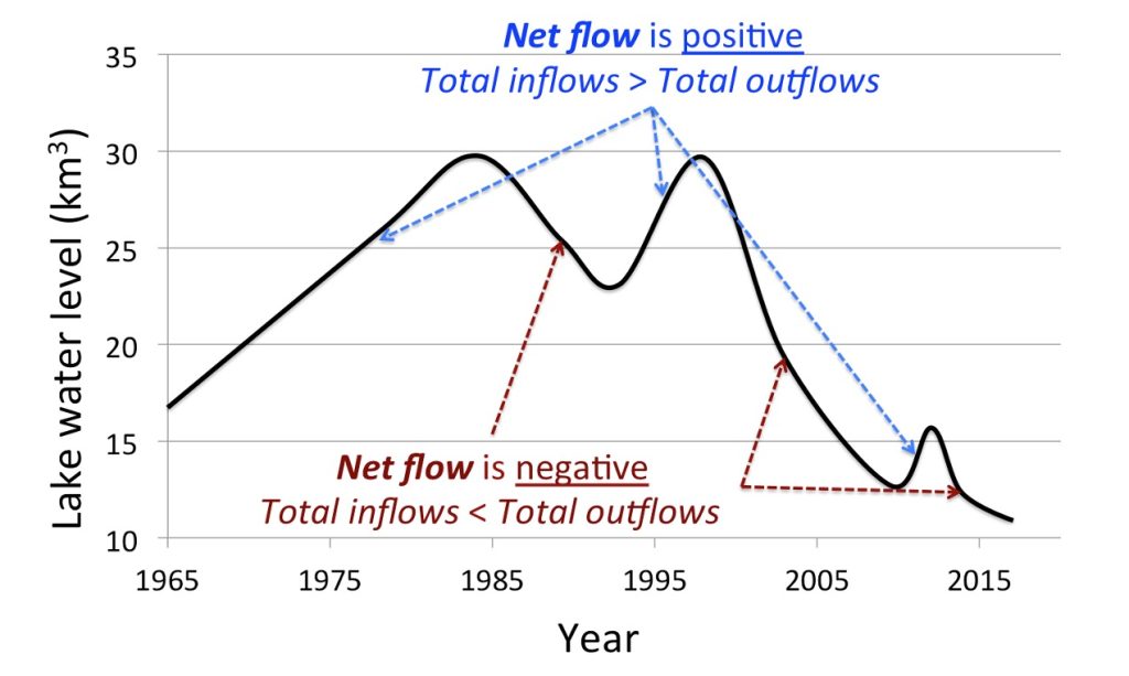
The bathtub analogy shows how the net flow in Figure 12 affects the water level in Lake Mead.  Figure 13 shows a smoothed version of the Lake Mead water level and shows the common-sense relationship between Lake Mead’s water level over time and its net flow.  As long as the net flow is positive, water is flowing into the lake faster than it is being removed; the water level will rise. On the other hand, if net flow is negative, water is flowing in more slowly than it is being removed; the water level will drop.

3.3. A Step Through Time: Simulating a Stock’s Behavior Using a Net Flow

The common-sense relationship between a stock and its net flow provides the key by which a computer simulation model calculates (i.e., simulates) both past and future contents of any stock.  Fortunately, these calculations are quite simple.

Suppose it’s August 2 in 1995. The latest measurements indicate that the water volume in Lake Mead is 25 cubic kilometers of water. If you want to calculate how much water you think will be in Lake Mead one year from now at the beginning of 1996, what is a reasonable way of doing that?  We can’t read the future, but we can make some educated guesses that would help us make the required calculation. In particular, since we know that the level in a stock can be affected only by that stock’s attending flows, it stands to reason that, if we had a reasonable guess of what the flows would be during 1995, we’d be able to figure out (somehow) what the water volume in Lake Mead would be one year from now. Suppose that we have the following predictions of what these flows would be over the next year.

• Inflow of Water Flowing In: approximately 12 km3/yr
• Outflow of Evaporation: approximately 1.5 km3/yr
• Outflow of Water Withdrawn for Human Use: approximately 2 km3/yr
• Outflow of Water Released Downstream: approximately 11.5 km3/yr

Based on these figures, we can figure out how much water would be in the lake one year from now. We simply calculate the net flow into Lake Mead by adding to the current contents of the lake (i.e. 25 km3) all of the inflows over the year and subtracting out all of the outflows. This gives (25+12-1.5-2-11.5) = 22 km3.  Another way of thinking about this is that we add to the current lake volume the net flow of water over the next year, where the net flow, as calculated in Figure 12. The total inflows are 12 km3. The total outflows are 1.5 + 2 + 11.5 = 15 km3. The net flow is 12 – 15 = -3 km3.  Hence, the predicted lake volume one year from now is 25 + -3 = 22 km3.

What if we wanted to calculate the water level only 6 months into 1995?  Then we could take ½ of the annual net flow (since the net flow gives the net amount of water added or removed over a full year). Since the net flow for a year is -3 km3. We’d expect the net flow for ½ year to be -1.5 km3. Hence, the predicted lake contents after one half year would be 25 + -1.5 = 23.5 km3.

This illustration leads us to the following principle for calculating stock levels based on the net flow.

Notice that we don’t just add the net flow to the current value of the stock. Since the net flow gives the amount added to the stock in one full time unit, we scale the net flow by multiplying it by the size of the time step over which we desire to simulate changes in the stock. In the case of the Lake Mead example, if we are simulating one year ahead, then = 1 year, and we add in the net flow. If we are simulating the stock value only six months ahead, then = ½ year, and we add in ½ of the net flow.

To see how the difference equation is used to simulate the behavior of a stock over time, let’s look at a very simple scenario with the Lake Mead stock and flow model.  Suppose that it’s 1995 and the contents of the lake is 25 km3 of water. Further suppose that, over the next five years, the flow rates are constant at the same values given earlier.

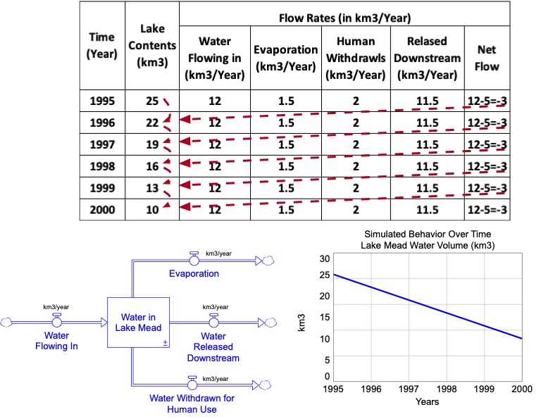
Using the simple rule for calculating future levels of the stock, based on the net flow, we can simulate changes in the water volume in the lake over the next five years. Figure 14 shows these calculations and the resulting behavior over time graph. The table begins with the initial lake contents of 25 km3. The lake content in subsequent years is calculated using the value from the previous year and the net flow during the current year.  The dashed arrows show which values are used to calculate the values for the next year.

One can see from the table in Figure 14 that the net flow is a constant -3 km3 each year, indicating that the lake would lose 3 km3 of water each year. This constant rate of loss is seen in the graph below the table, where the contents of Lake Mead shows a linear trend with a slope of -3 km3/year.  What if the net flow had worked out to be a constant increase of 3 km3/year? Then the graph would still be linear, but would have an upward slope of 3 km3/yr.

The example in Figure 14 is very simplistic because it assumes that the rates of all four flows associated with Lake Mead remain constant over a five-year period. We know that this cannot be true. For example, the water flowing into the lake via the Colorado River will naturally vary from year to year, depending on amount of rainfall that year, as well as the amount of water taken from the river by people upstream. Likewise, the amount of water released downstream, the withdrawals by humans, and the evaporation rates are all subject to fluctuations in weather, human need, and many other factors.  Hence, any useable simulation model must be able to account for these kinds of ever-changing conditions.

For now, we’ll not concern ourselves with incorporating human activity, and other factors into the model. Instead, we will restrict our attention on how a simulator would calculate the stock of Lake Mead water volume from year to year whenever the flow rates do change. The good news is that this is still done using the simple approach illustrated in Figure 14.

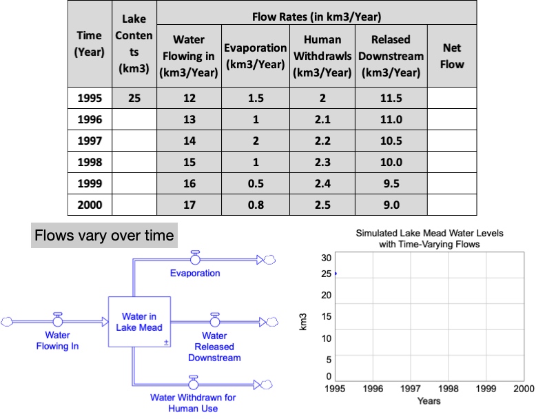
As before, assume that it’s 1995 and the contents of the lake is 25 km³ of water. This time, however, let’s assume that the flow rates vary over the next five years as follows.

• Inflow of Water flowing in: Currently 12 km³/yr, but increasing by 1 km³/yr.
• Outflow of Evaporation: fluctuates randomly (because of multiple factors). It is 1.5 km³/yr during 1995; in the next five years it is 1 km³/yr, then 2 km³/yr, then 1 km³/yr, then 0.5 km³/yr, and finally 0.8 km³/yr in 2000
• Outflow of Withdrawal by humans: humans currently remove 2 km³/year in 1995. However, due to increases in population, the annual consumption rate increases by 0.1 km³ every year.
• Outflow of Released downstream: 11.5 km³ per year are released downstream in 1995, but decreases by 0.5 km³ each year after that.