4 Chapter 4: Introduction to System Dynamics Modeling
Now it’s time to apply what you’ve learned to begin building simulation models that mimic many of the feedback dynamics in complex problems like the Kaibab ecosystem. This chapter will lead you through a series of model building exercises that provide building blocks that are useful in a wide variety of real-life situations, including the problems on the Kaibab Plateau. Along the way, you will learn some of the basics of system dynamics model building. For each exercise you will build a running simulator of a simple system. Your model will include appropriate graphs and simple user interface features to allow you and others to experiment with the model. We’ll use Stella Architect®, created by isee systems, as the model-building platform, but these models could be built using any system dynamics modeling software packages. The sequence of models you will build over the next few weeks are listed below.
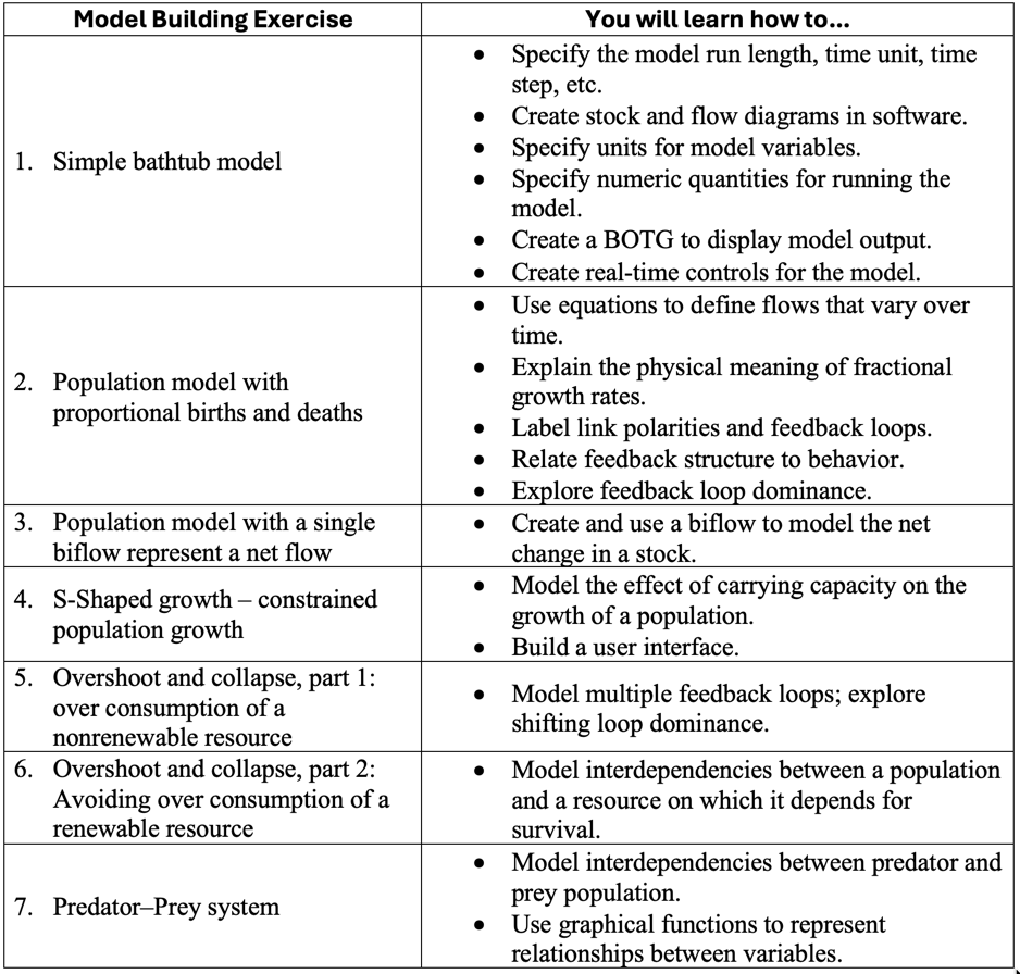
4.1. A Simple Bathtub Model: Behavior when Flows are Constant
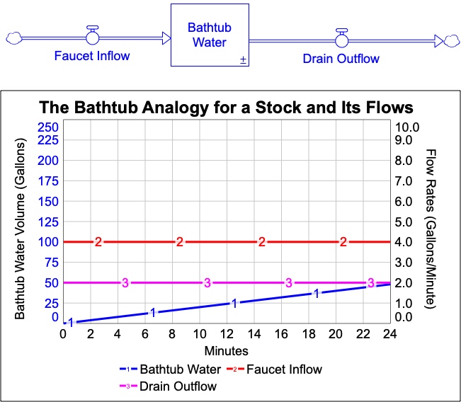
Figure 4.1 shows the stock and flow diagram and an associated BOTG that you will create for your first model. The stock and flow structure is a system dynamics representation of the bathtub analogy in Figure 2.9. The BOTG shows the amount of water in the bathtub (left axis) and the flow rates in the faucet and drain (right axis).
Exercise 4.1: Modeling Challenge – Build the Bathtub Model
Part 1: Building the model
You will build this model in Stella Architect®. As you complete this activity, use the following checklist to make sure you learn the skills required to move on to the next model activity. Check off those items that you know how to do. Your instructor can help with those items about which you are uncertain.
- ❏ Explain the meaning and purpose of the following, and set their numeric values.
- ❏ Start time (set to 0), stop time (set to 24)
- ❏ Time unit (select “minutes”)
- ❏ Time step (set DT to be a fractional value of ¼ minute)
- ❏ Simulation duration (set to 10 seconds)
- ❏ Create and name the stock; add the flows and connect them to the stock; name all the variables (follow Figure 4.1).
- ❏ Set font size for stock and flow names to 14 pt font
- ❏ Designate the units for the stock and its flows
- ❏ Document a physical description of each variable
- ❏ Specify the numeric quantities for the flows and for the starting value of the stock (set the inflow rate to be 4 gal/min; outflow to be 2 gal/min; bathtub starts empty)
- ❏ Add a BOTG showing the water in the bathtub stock and the values of the two flows. Provide a meaningful title and left + right scales for the graph as in Figure 15.
- ❏ Specify input limits for the values of the flows (set min and max for each flow to 0 and 10 gal/min, with incremental adjustments of 0.1 gal/min)
- ❏ Run the model and vary the flow values to see how they affect the BOTG.
Part 2: Exploring the model
Once you have completed all of the above, use your model to answer these questions.
- Initially, what is the value of the net flow into the stock before you make any changes?
- Under what conditions of the net flow does the water in the tub rise? Under what conditions does the water level drop?
- Now run the simulator. About ½ way through the simulation, use the control slider on the inflow (faucet) to set the inflow to zero. What happens to the BOTG of the stock after this? Use the net flow to explain the shape of the particular pattern you see.
- Click the RESET button (the “U-turn arrow” at the bottom left of the Stella modeling screen) to restore all the flows to their original values, then run the simulator again, but this time, about ½ way through, move the outflow (drain) to zero. Answer the previous question again for this new experiment.
- Does this model include any feedback? Explain.
Part 3: Making a Causal Loop Diagram
Draw a CLD for the bathtub model. Label the polarities of all causal links, as well as the polarities of any feedback loops you find (if any). For the purposes of this exercise, draw your CLD without including symbols for stocks and flows. Your CLD should have three variables in it.
4.2: Constants, Initial Values, and Equations
No matter what simulation modeling software you are using, the software will take care of the difficult math for you. Your job is to figure out the calculations between variables and the values for constants, nonlinear functions, and the initial conditions of stocks.
Each stock needs an initial condition or starting value. The stock in the bathtub model starts at zero. There is no water in the bathtub when the model starts to simulate. If I were looking at the world population and starting my model in 1950, I would go to a reliable source, perhaps the Population Division of the United Nations, and get data. The world population in 1950 was approximately 2.5 billion people. I would use this value as the initial condition of my population stock. All stocks need an initial value or starting condition. You can make the initial value of a stock a function of another or a combination of other variables in your model. We will show you some simple examples later in the text. You will not need them now.
Constants are values that are not affected by other variables in the model. An example would be the number of Miles Driven per Year per Vehicle. The Federal Highway Administration data indicates that this is 14,500 miles per vehicle per year. If you multiplied this by the number of Vehicles, you would be able to calculate the Total Miles Driven per Year. New information may come along, and the value of the constant could be changed. You could also vary this value to determine what would happen if more or fewer miles were driven per vehicle each year. The only rule with constants is that you should not add them to a model simply to make the units correct.
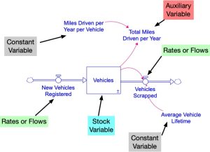
An auxiliary variable is calculated from other variables in the model. In the example in Figure 4.2, the variable labeled Total Miles Driven per Year is an auxiliary variable and is calculated by multiplying Miles Driven per Year per Vehicle (a constant) times Vehicles (a stock). Auxiliary variables are going to be calculated by multiplying, dividing, adding, subtracting, or some combination of these operations. This also applies to rate (flow) equations. Technically, all auxiliary variables are rate equations in that auxiliary variables will flow back to change rates (flows) into and out of all stocks (Forrester, 1961).
The other type of equation showing up in a model is a nonlinear or graphical equation. These are used when the output of a variable does not change proportionally to the input and this will be discussed in detail later.
Exercise 4.2: Team Modeling Activity – Applying the Bathtub Model
This is the first of several group model building challenges you will encounter throughout this Learning Guide. The purpose of these challenges is to give you practice in three things:
- Recognizing how the models built in other exercises can be applied to different contexts.
- Adapt those models to create stock and flow diagrams and model equations for those contexts.
- Work with others to accomplish all of this.
We identify these activities as TEAM Modeling Activities because they require you to “think in systems” with others. System dynamics modeling is a team sport! The expertise, perspectives, and skills of multiple people are needed to successfully create a model that is useful to decision makers. By learning how to work alongside others, you will learn how to use systems thinking terminology and how to make sure you don’t miss important features of the system. If you continue your studies in systems thinking, you may eventually find yourself participating in or leading a group modeling session with stakeholders and experts who know the system, but don’t know how to use systems thinking (Andersen and Richardson, 1994; Vennix, 1996, Hovmand, 2014). That is a challenging and very rewarding experience!
To do each Team Modeling Activity, you will work in teams of 3-5 people during class time in order to complete the assignment. Your instructor will be present to help if your team gets stuck, but not to give you the answers!
Instructions
Each example below describes a different situation in which The Bathtub Model (Figure 4.1) can be adapted to each of the systems described below. In each case, sketch out on the wall (using a white board or poster paper) the stock and flow structure for the indicated system. Give the stocks and flows names corresponding to the context. Then write on the wall the equations for each flow, and the starting values for the stocks. Then build the model in Stella®. In each case, your model will involve one or more stocks and one or more flows, where the flows are constants.
- At the start of the semester, your bank account contains $1500 dollars. Each month you get $400 from your part-time job. Your share of the rent and utilities is $350/month, and you spend $100/week on groceries, gas for your car, and extracurricular activities. What happens to your bank balance over the next nine months?
- In 2008 there was 2996 billion metric tons of carbon in the atmosphere. Every year, human activity releases 9.1 billion tons of carbon into the atmosphere. 5 billion metric tons are removed through absorption into plants (i.e., photosynthesis), the ocean, and soil or rocks. Assuming these rates remain constant, how much will the atmospheric carbon change between 2008 and 2108.
- You currently have a backlog of 5 homework assignments that you must complete and turn in. Each week, you get an additional 7 assignments, and you complete 5 assignments. What will happen to your backlog over the next 10 weeks?
4.3. A Simple Population Model: Behavior When Flows Vary Over Time
The purpose of the bathtub model exercise was to introduce you to some of the basic concepts used in building running simulators involving stocks and flows. Of course, most problems of interest (like the Kaibab, for example) do not involve bathtubs, faucets, and drains. In the case of the Kaibab, the stocks of interest are populations of animals and plants.
In fact, many system dynamics models involve stocks of populations of various types. The next several modeling exercises will introduce you to some of the fundamentals for modeling population dynamics. We’ll begin with a simple population model: one that involves births and deaths. In later exercises we will add more complexity to the model by considering how births and deaths are impacted by limitations of the surrounding ecosystem, by the presence of predators, and by consumption (or overconsumption) of limited resources.
Imagine a population of people in a region filled with abundant food and other resources necessary for that population to flourish over the foreseeable future. In this idyllic situation, let’s assume (for simplicity) that there is no threat of starvation, disease, war, or other factors that could alter the basic dynamics created by the processes of birth and death.
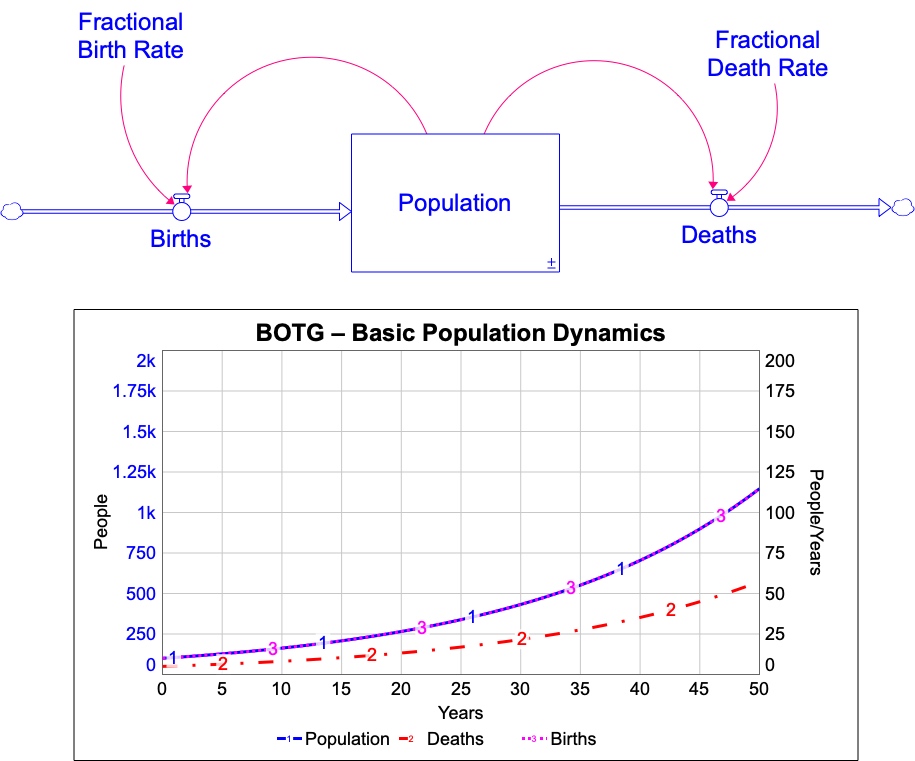
Figure 4.3 shows the stock and flow structure (and behavior over time) of this simple, idyllic population. This stock and flow diagram matches the structure we used for the deer population in Figure 2.10. As in that figure, there are two feedback loops in this system. You will shortly get a chance to identify those loops and explore their role in the system.
4.3.1. A Word About the Unit of Time
Because we are modeling a human population over time, we do not need to track the population size every second, minute, day, or probably even every month. Instead, we can probably use a time unit of one year for our simulation. Hence, all of the flows in this model will be expressed as the number of people added to or removed from the population over a given year.
4.3.2. Fraction Birth and Death Rates
Figure 4.3 includes two new variables that require some explanation. These are the Fractional Birth Rate and the Fractional Death Rate. In general, these represent the fraction by which the Population changes because of births or deaths in one time unit of the simulation (in one year). For example, a Fractional Birth Rate of 0.10 means that the Population will grow by 10% each year – all because of births. This is equivalent to saying that 10% of the population will have a child born during the next year. That’s why the Fractional Birth Rate is sometimes called the per capita birth rate. On the other hand, a Fractional Death Rate of, say, 0.05 means that the Population will shrink by 5%, from what it would have been, because of deaths (i.e., 5% of the Population will die over the next year). The Fractional Death Rate is sometimes called the per capita death rate.
The units for these quantities are not immediately obvious. One way to determine the units for these quantities is to think about how they are used to calculate the two flows in the diagram. Given the physical explanation of the Fractional Birth Rate in the previous paragraph, it is clear that, to calculate the number of births in a given year, we just multiply the Fractional Birth Rate by the Population. For example, if there are currently 1000 people in the Population and the Fractional Birth Rate is 0.05, then over the next year we would expect to see Births that increase the Population by 5%. That means there would be an inflow of 0.05*1000 = 50 people via the Births inflow. In general, this translates into the following equation for calculating the Births inflow:
Births = Fractional Birth Rate * Population
However, we also know (from the earlier discussion about unit compatibility) that, if the units for the Population stock is measured in people, then the units for the Births flow must be measured in people/year. By substituting these units into the above equation we see that:
Units for Births flow = Units for Fractional Birth Rate * Units for Population
people/year = Units for Fractional Birth Rate * people
This means that the units for the Fractional Birth Rate must be 1/year (aka fraction/year, dimensionless/year, or 1/year) in order for the units on the right side of the equal sign to work out to be people/year.
Using the same reasoning, the units for the Fractional Death Rate will also be fraction/year.
Exercise 4.3: Build the Basic Population Model
Part 1: Build the model
Build the basic population model in Figure 4.3, including the BOTG. Your graph’s output should exactly match what you see in Figure 4.3.
- Model Settings
- Start time: 0
- Stop time: 50
- DT = 1
- Sim duration: 1.5 seconds
- Time units: Years
- Add the feedback loop indicators with R & B notation. Number the R’s and B’s to uniquely identify each loop (i.e., R1, B1, R2, B2, etc.).
- Give descriptive names to each of the loops.
- Set up the feedback loop indicator so that, when you place your cursor over the feedback indicator, all the variables and links in the loop are highlighted. Do this by double-clicking on the circular feedback loop indicator and selecting which variables are included in the feedback loop.
- Label all causal links and flows with +/- causal link polarities.
- Use 14 pt font for all variables, graphs, etc.
- Use the following values for the variables, stock, and flows in the model.
- Population: set the initial value to 100 people
- Births: set equal to Population*Fractional Birth Rate
- Deaths: set equal to Population*Fractional Death Rate
- Fractional Birth Rate = 0.10; fix slider Input range to be min=0; max =0.2
- Fractional Death Rate = 0.05; fix slider Input range to be min = 0; max = 0.2
- Specify the units and physical descriptions for all of the variables and check that you have no errors in units.
Part 2: Explore the model
- Explain why each loop is the type you indicated. That is, if the loop is reinforcing, explain how that loop works to “build momentum” toward faster and faster growth. If balancing, explain how that loop works to check or compensate against growth away from some equilibrium.
- Make sure your model produces the exact same BOTG as shown in Figure 4.3.
- Use your running model to answer these questions
-
- How would you calculate the net flow for the Population stock?
- Using the original values for the Fractional Birth Rate and Fractional Death Rate, run the model. Based on the BOTG, which feedback loop dominates this system? Explain.
- Now, run the model and vary the Fractional Birth Rate and Fractional Death Rates. Under what conditions does balancing feedback dominate this system? When does reinforcing feedback dominate this system?
- Now change the DT to 1/12 year in your model, so that it calculates the population values every month instead of once/year. Run the model and compare the output to what you got from the original run when DT was set to 1 year. Why did you get different results? Which do you think is more reliable? Why?
Exercise 4.4: Apply Your Model to World Population Projections
Now apply your model to the world population, starting in 1950. The graph below (from the United Nations) shows the BOTG from 1950 through 2100. The values from 1950 through 2016 are official UN world population estimates. The values beyond 2016 are projections based on the UN’s population models. The three curves (labeled as the “Low,” “Medium” and “High” variants) show three different behaviors over time that could emerge between 2016 and 2100.
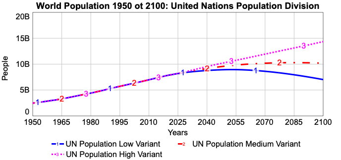
- Of the three curves in the graph, which curve (or curves) do you think represent the UN’s “hopes” for the future? Which curve (or curves) represent the UN’s “fears” for the future. Be ready to explain your answers.
- Now, adapt your population model to see how well it matches the UN’s projections in the above graph. Do this by changing units for the Population stock to people. Change the units in the two flows to be compatible with any change in the stock units. Adjust the Run Specs on the model to start in 1950 and run through 2100. Also, adjust the DT value so that the module updates the population every month. Set the Population to start at 2,471,424,000 people: the population in 1950.
- Run your model and adjust the Fractional Birth Rate and Fractional Death Rate for the world population to match as closely as you can the BOTG up through 2016 in the figure above. Use the actual population values in the lower right box as a check. Hint: Try setting the Precision on the input ranges for these two variables to be 0.001 to allow finer adjustment of these variables.
- Record the Fractional Birth Rate and Fractional Death Rate that best match the UN curve up through 2016. How do you feel about these fractional values in terms of their appropriateness for a human population? Can you find data on the web to give you an idea of what these values are in practice?
- Can you find other values for these fractional rates that will produce the same BOTG that you got in #4. Explain.
- How does the resulting simulation BOTG compare to the UN historical trends up through 2010? How does your model’s output compare to the projected trends beyond 2016? What issues do you see?
- What does the resulting BOTG from your model (with the Fractional Birth Rate and Fractional Death Rate you’ve chosen) suggest about the world population through 2100? How does this differ from the UN’s model? How do you feel about the accuracy of your simulation? Explain.
4.2.3 Applying the Basic Population Model to Other Contexts
In the previous section, you learned that the birth and death flows in the basic population model are calculated as follows:
Births = Population * Fractional Birth Rate
Deaths = Population * Fractional Death Rate
That is, the two flows are determined by multiplying the stock by a numeric constant (the Fractional Birth Rate or the Fractional Death Rate). Hence the flows are proportional to the size of the stock because they are calculated by multiplying the stock by a constant (the fractional birth or death rate).
This proportionality relationship is a commonly occurring relationship between a stock and its flows. Whenever you are building a stock and flow model, if you believe that the flows depend on the size of the stock, a good place to start is to see if a proportional relationship makes sense.
For example, consider how the level of support for a particular political cause might be modeled. Figure 4.4 shows a logical stock and flow model for this phenomenon.
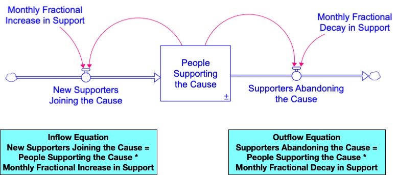
Notice that this model looks just like the simple population model in Figure 4.3. The only evident change is in the names of the stock, flows, and fractional rate constants. Furthermore, the flows in this model would be calculated the same way as in the population model: by multiplying the stock by the indicated fractional rate constant.
Now let’s return to the original population model to further explore other forms that proportional stock and flow relationships can take. Suppose, for example, that we do not know the fractional death rate in the model, but we do know that people in this population live for 80 years, on average. Can we use this to calculate the death outflow? The answer is yes! Since the average lifespan is 80 years, we know that every year about one-eightieth of the population will die. In other words, the death flow would be calculated by dividing the population by the 80-year lifespan. In equation form, the equation for the death outflow would be as follows.
Deaths = Population / 80 (Average Lifespan),
or equivalently
Deaths = Population * 0.0125, since 1/80 = 0.0125.
Now consider a lake that has water flowing into it (via a stream) and flowing out of it (via the extension of the same stream). Further suppose that we know that water flows into the lake at a rate of 1000 gallons per day and that, because of mixing, each drop of water remains in the lake for, on average, 20 days. The 20-day residence time is analogous to the 80-year lifespan in the population model. That is, each day, one-twentieth of the water in the lake will flow out and downstream. The stock and flow model for this situation is given below in Figure 4.5.
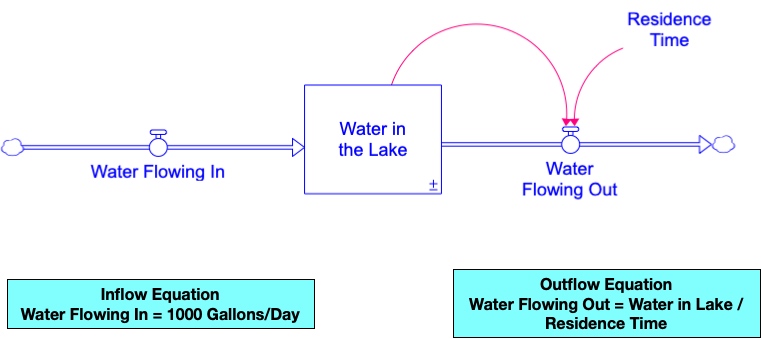
Notice that the outflow is proportional to the stock. It is calculated by dividing the stock by the Residence Time. Also notice that there is no causal link pointing from the stock back into the inflow. That’s because the inflow rate is a constant 1000 gal/day; it doesn’t depend on the amount of Water in the Lake.
Exercise 4.5: Team Modeling Activity: Other Applications of the Population Model
You will work in teams of 3-5 people during class time in order to complete the challenge. Your instructor will be present to help if your team gets stuck, but not to give you the answers!
Each example below describes a different situation in which the population model (Figure 4.3) can be adapted to a new context. In each case, do the following:
- Sketch out on the wall (using a whiteboard or poster paper) the stock and flow structure for the indicated system.
- Give names to the stocks and flows that correspond to the context.
- Write on the wall the equations for each flow, and the starting values for the stocks.
- Then build the model in Stella®. In some cases, you may need to eliminate one of the flows or add an additional stock and corresponding flows.
- Once you build each model, draw a simple Causal Loop Diagram (without drawing stocks and flows) showing the feedback loops in the system. Be ready to use your CLD to tell the story about how the feedback structure drives the behavior of the system.
Here are the different situations for you to model.
- In 2013, there were 90 million Instagram users. Since that time, the number of new active users has grown annually by about 30%, and 5% of existing users have either cancel or don’t use their account. What will happen to the number of users through 2030, assuming these rates continue?
- An investor has stock market investments that grow in value by an average of 4% each year because of market growth. Each year, the financial investment company managing that investor’s account charges the investor 0.5% of the total investment worth in order to pay for their services. Assume that the investor starts with $10,000 in the account. How will the value of the investor’s holdings change over the next 30 years?
- Radon-222 is a radioactive gas that is fairly common in underground wells of water, the soil or rock deposits. It can percolate into the basement of a home that is built over radon-containing soil. As it decays, it can emit radioactive particles into the home, endangering the health of its inhabitants. Fortunately, radon eventually decays into lead, which is not radioactive. Each day, 18.3% of radon decays in this way. Draw a stock and flow diagram (with fractional birth and/or death flows) of a 100 kilogram (kg) radon deposit located in the soil under a residence to model the Radon’s decay into lead. Experiment with this model to figure out how long it takes for half of the radon to decay. Use different DT values from a DT of 1 to a DT of 50 and see how your answer changes. Explain.
- The nation of Camazy currently has a population of 301 million people. 75 million of them are 20 yrs old or younger; 76 million are between 21 and 45, and 150 million are over 46. Only those who are between 21 and 45 bear children. While at childbearing age, the birth fraction in this age group is 0.04. That is, to calculate the number of births each year, you must multiply the number of people aged 21-45 years times the 0.04 birth fraction. Each year, 3% of the oldest group dies, while 1% of the two youngest groups die. Create a stock and flow model for the Camazy population over the next 3 centuries. In your model, you will have three stocks (one for each age group) and flows connecting one age group to the next. Set the stock units to be thousands of people (so that 75 million people would be 75,000). Use exogenous variables that will allow you to adjust the birth fraction and two death fractions. Use a DT of ¼ year. What is the future of Camazy over the next 300 years? Find conditions under which the Camazy population does the following: (i) levels off, (ii) grows continually or “explodes,” and (iii) declines or “collapses.” Explain what is happening.
- Every year, a county landfill leeches 20 tons of toxic chemicals into the soil. It takes about 3 years, on average for these chemicals to make their way into the local underground aquifer. Once in the aquifer, the chemicals travel downstream until they reach a reservoir that provides water to a large community. It takes about 10 years, on average for the chemicals to travel from the aquifer below the landfill to the reservoir. Once in the reservoir, the toxins either flush downstream or are forever chemicals and remain in the environment. About 5% of the toxins making it to the reservoir are forever chemicals. The residence time of water in the reservoir is about 18 months (1.5 years). Build a model with the stocks below (start all stocks with 0 tons of toxins). Add the flows, their units, and the equations to calculate them. Create a BOTG showing all four stocks. Run your model for 100 years (with a DT of ¼ and a Sim Duration of 10 seconds to allow you to adjust model parameters in real time).
-
- Toxins in the Soil
- Toxins in the Aquifer
- Toxins in the Reservoir
- Forever Chemicals Remaining in the Environment
- Terrorist groups work hard to recruit individuals to their cause. In a given country, people begin as “potential recruits.” Every month, based on the recruitment activities by the terrorist organization, about 1% of potential recruits become sympathetic to the cause, while another 0.75% are “turned off” and become immune to recruitment. Of those who become sympathetic, each month, 5% of them become full converts to the terrorist cause and 0.75% are “turned off.” After becoming full converts, 2% become disillusioned and “turned off” each month. Once someone is a full convert, their life expectancy is 10 years before they are caught or killed by counterterrorism forces. Build a stock and flow model in Stella with these stocks. Document the equations and units of all flows. Create a BOTG showing the stocks below. Run the model for 240 months.
-
- Potential recruits (start with 15,000)
- Turned off to the cause (start with 0)
- Sympathetic to the cause (start with 0)
- Full converts (start with 20)
- Terrorists caught or killed (start with 0)
- Each year the U.S. Drug Enforcement Agency (DEA) recruits 1000 new agents to join its ranks. These agents spend, on average, 12 months in training before being deployed to the field. 2% of new agents “wash out” of the training in the 1st 12 months. After training, the recruits are transferred to active duty. Agents stay on the job, an average of 20 years; however, if corrupted, they last an average of only 15 yrs before being either convicted, killed, or retiring. Every month, 1/10 of a percent of active agents are “turned” toward corruption to work for drug cartels while on duty. Every year, about 2% of agents are injured on the job. These agents are off-duty for 3 months, on average. Create a model in Stella® using the following four stocks. Make a BOTG showing the behavior of the stocks over a 50-year period. Based on the simulation time you pick to run the model, you may have to perform some calculations so the data provided is in the appropriate time format.
-
- New agents in training (start with 500 new agents)
- Agents on active duty (start with 9000 active agents)
- Corrupt agents (start with 0 corrupt agents)
- Injured agents in recovery (start with 0)
Which flows are proportional to the stocks? Which are not?
4.3. Reflecting on Model Validity: When is a Model “Good Enough?”
In Exercise 4.4, you used a UN-based BOTG on world population to help you choose values for the starting value of the Population stock, as well as for the Fractional Birth Rate and Fractional Death Rate. This is a common practice in modeling: using historical data to help us “tune” the parameters in the model and then checking to see how the model matches the past and whether it produces future behavior that we think is reasonable. You probably noticed a few issues as you worked on that exercise.
- Inappropriate behavior over time. Your simple population model cannot produce the historical curves nor the “hopes and fears” curves produced by the UN model. In fact, the only behavior your model can produce is exponential growth or exponential decline (depending on what values you set the Fractional Birth and Fraction Death Rates). Because the UN model is based on real historical data, and because it is produced by expert population modelers, it suggests that the simple feedback structure in your model does not capture the feedback structure used in the UN model.
- Indeterminate parameter values. You may have noticed that there are many combinations of values for the Fractional Birth Rate and Fractional Death Rate that produce the same BOTG. The next Modeling Challenge shows several pairs of Fractional Birth and Death Rates, where each produces the exact same BOTG.
Exercise 4.6: Modeling Challenge – The Problem of Indeterminate Parameter Values
| Candidate Pair | Fractional Birth Rate | Fractional Death Rate | Fractional Net Growth Rate |
| 1 | 0.05 | 0.048 | |
| 2 | 0.02 | 0.00 | |
| 3 | 0.04 | 0.02 | |
| 4 | 2.10 | 2.08 |
The above table shows Fractional Birth and Death Rates. Try these values in your basic population model and you will see that each pair produces the exact same BOTG. Calculate the fractional net growth for each pair (i.e., Fractional Birth Rate – Fractional Death Rate). How does this explain why these pairs all give the same BOTG? Which pairs should be ruled out as unreasonable for a human population?
The two issues of inappropriate behavior over time, and indeterminate parameter values are common, but necessary challenges when we build models of dynamic systems. During every step of the modeling process, we should test our model’s validity to see if it produces behaviors that we know should be present in the system. We also check to see if the numeric quantities we are using in the model are, reasonable, given the context of the problem. There are many other validity tests that need to be done (Sterman, 2000; Barlas, 1996; Forrester and Senge, 1980, Greenberger et al., 1976), but those are beyond the scope of this text. However, when we test model validity and see problems, we probably need to make some changes to the model!
However, we can never get a perfect model…one that provides precise output that we can quote with absolute confidence. That’s because a model is a simplified version of reality. It inevitably involves compromises. We make choices about which details from the real system to include in the model, which to ignore, and which to include as a sufficient approximation to reality. Otherwise, if we try to build a perfect model, we’ll never finish, and our model will be too complicated to be understandable or useful. Just what constitutes a “good enough” model is a difficult question to answer, and one that requires more time and effort than is appropriate at this stage. However, we can keep in mind a profound and simple quote from one of the great modelers and statisticians of the last century, G.E.P. Box (1976).
This statement provides a rough guide to modelers of all types. To be “good enough” a model must be useful to those who depend on it to help them make decisions. A model need not provide perfect predictions. It does need to provide predictions that are good enough to help a decision maker know what sorts of conditions could lead to system behavior that reliably mimics their hopes or their fears. Given such a model, along with a knowledge of how the feedback structure in the model works to create that behavior, a leader is in a much better position to make interventions that produce the desired results.
It is clear that a simple population model is not “good enough” to give us insights about the future of the world population. In fact, it’s not good enough to model most real-life populations, including those of plants, animals, bacteria…you name it. We know that no population of living organisms can grow exponentially forever (Meadows et al., 1972).
Hence, we now turn our attention to ways our simple population model can be expanded to account for dynamics that constrain unfettered growth thereby causing the population size to eventually level off, or decline or maybe even oscillate over time. But before we can accomplish this, we must first address the problem of indeterminate parameter values. We will show a way to simplify the simple population model to help with this issue.
4.4. The Simple Population Model Revisited: Using a Biflow
We’ll begin by tackling the problem of the indeterminate parameter values that you saw when you tried to find values for the Fractional Birth Rate and Fractional Death Rate to match the United Nations BOTG in the previous Modeling Challenge (Exercise 4.4).
One of the problems with finding the correct values for the Fractional Birth Rate and Fractional Death Rate is that many times the data we have about a population gives us only the fractional net growth rate. For example, here are a few lines of data from the United Nations used to make the World Population BOTG you saw earlier (United Nations, Department of Economic and Social Affairs, Population Division, 2022).
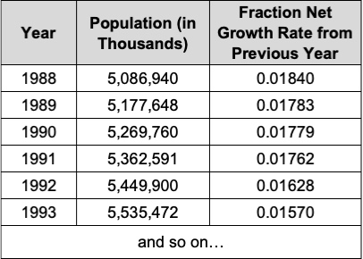
Notice that, for each year, this table shows the number of people (in thousands) and the Fractional Net Growth Rate from the previous year. To get the Fractional Net Growth Rate for a given year, we calculate how many people were added since last year and express that value as a fraction of last year’s population. For example, the Fractional Net Growth Rate from 1990 to 1991 is (5,362,591 thousand – 5,269,760 thousand)/(55,269,760 thousand) = 0.01648 or 1.648%. That is, the population grew by 1.648% from 1990 to 1991.
With population data, we seldom know the Fractional Birth Rate and Fractional Death Rate, but we can often use historical data to calculate the Fractional Net Growth Rate. In addition, it turns out that the Fractional Net Growth Rate is the difference between the Fractional Birth Rate and the Fractional Death Rate, i.e.:
Fractional Net Growth Rate = Fractional Birth Rate – Fractional Death Rate.
You saw in in the previous Modeling Challenge (Exercise 4.6) that the Fractional Net Growth Rate determines the growth trajectory of the population. Hence, if we know the Fractional Net Growth Rate, we don’t need to know the Fractional Birth Rate and the Fractional Death Rate. Instead of separate birth and death flows, we can use a single Fractional Net Growth Rate as shown in Figure 4.6.
Figure 4.6 shows the original population model with two flows and a revised version, where we’ve combined the Birth and Death flows into a single Net Flow that depends on the Fractional Net Growth Rate. Notice the arrows on both ends of this flow. This is a biflow; it can flow into or out of the stock, depending on whether the flow is positive or negative. As long as the Net Flow is greater than zero, the population will grow. If the Net Flow is negative, the population will shrink.

Exercises 4.7: Modeling Challenge – Use a Single Net Growth Biflow for the Population Model
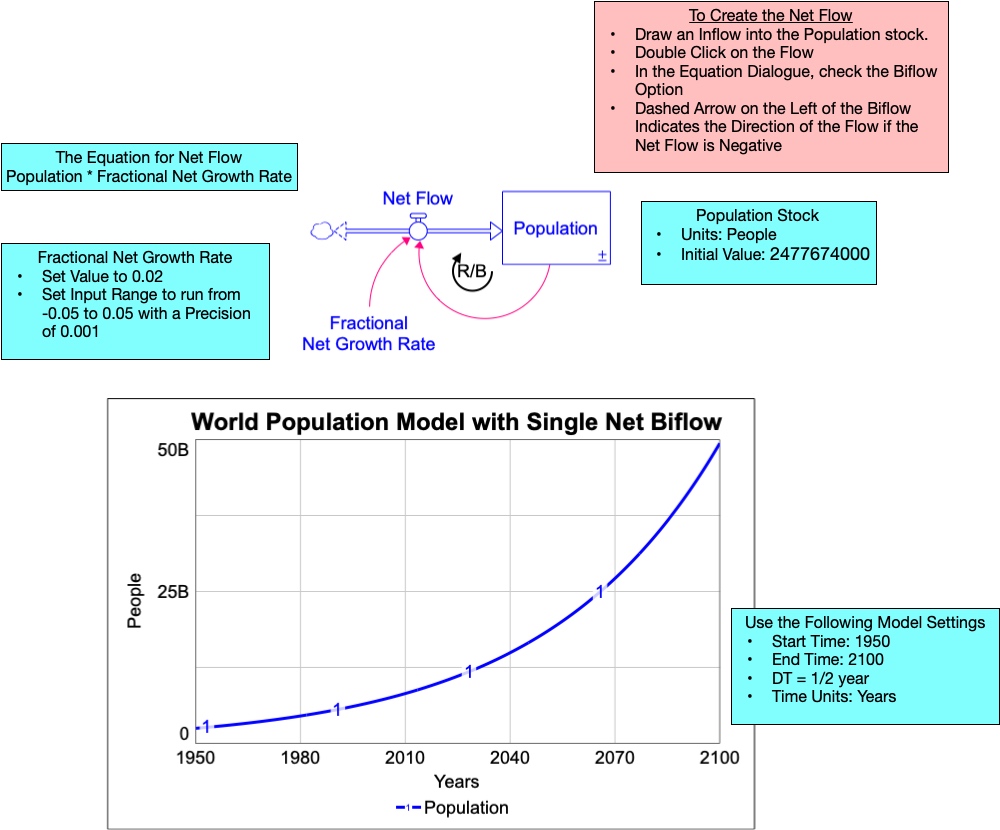
- Use the figure above to build the model of a population using a single biflow. Compare the BOTG with the original model with separate birth and death flows.
- Label the polarities of the red causal links and flow.
- There is now a single feedback loop in this model, and it is designated with a circular “R/B” notation, indicating that the loop could be either reinforcing or balancing. Under what conditions would this loop be a reinforcing loop? A balancing loop?
- What value of the Fractional Net Flow Rate best corresponds to the World Population BOTG shown earlier. How does this value relate to the Fractional Birth Rate and the Fractional Death Rate values that you chose in that previous action item?
- Refer back to the discussion about competing feedback loops and the earlier Modeling Challenge where you learned how the shape of a BOTG gives clues about when each type of feedback loop dominates the system. Now look at the BOTG in this latest population model. When the Fractional Net Growth Rate is positive, what kind of BOTG do you get? What type of feedback is dominating the system? What about when the Fractional Net Growth Rate is negative?
4.5. Modeling S-Shaped Growth – Population Growth Under Constraints
At this point, your population model still does not seem realistic. It suggests that the world population will keep growing exponentially up through 2100. In fact, as long as the Fractional Net Growth Rate is positive, the population will continue to grow exponentially. But this doesn’t make sense. After all, there is a finite amount of land area on the earth. There are finite resources such as water and food that can support a human population (Meadows et al., 1974). In addition, as the population grows, the impact of humans on those resources also grows. Over time, we would expect that humans might reach a maximum sustainable population. In addition, if we are not good stewards of the earth, we might overuse or degrade its natural resources. In that case, the world population could “overshoot” the capacity of the planet to sustain it. Then the world population would peak and eventually start to decline. The decline could be gradual or catastrophic, depending on the degree to which the planet’s resources have been degraded.
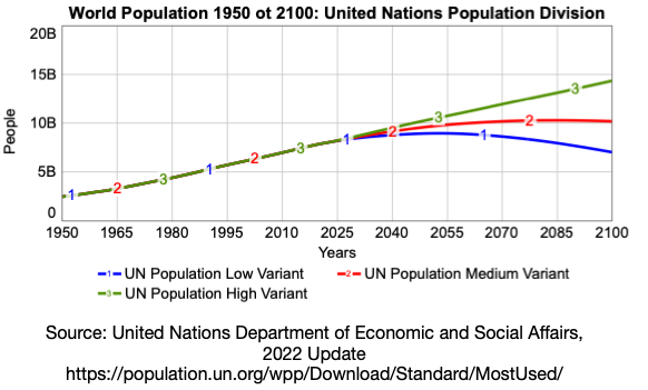
These two scenarios (growth to a sustainable population vs overshoot and collapse) are the same scenarios that the United Nations is concerned with. Figure 4.7 shows the same world population BOTG referred to earlier. Notice the three different scenarios or “variants” on this BOTG. We already know that the “High Variant” is not likely. The earth’s human population cannot continue to grow without bound forever. The “Medium Variant” curve corresponds to the case in which the world population reaches a stable, sustainable level. The “Low Variant” represents an overshoot and collapse scenario. From here on, we’ll refer to the “Medium Variant” curve as an example of S-shaped growth and the “Low Variant” curve as an example of overshoot and collapse.
Our goal in this section is to add feedback dynamics to our simple population model in order to mimic the S-shaped growth behavior over time. The resulting model will be based on what is known about the feedback dynamics affecting any population as it grows to a sustainable level.
Then we’ll turn our attention (in the next section) to adapting our S-shaped growth model to account for the case in which a population so degrades the resources on which it depends that it “overshoots” the sustainable population size and eventually starts to decline, or even collapse catastrophically.
Every population of living creatures depends on resources for its survival. Some of those resources are so abundant that we will not have to worry about over consuming them…at least for the imaginable future. Sunlight is an example of one such resource. It has taken the sun about 4.5 billion years to burn ½ of the hydrogen fuel it needs for nuclear fusion. That means that the sun will probably last for a few more billion years before its fuel is exhausted.
Other resources are not so abundant, but many of them are renewable. This means that they regenerate themselves over time, often on an annual cycle, but sometimes over much longer time periods. Food (either from animals or plants) is one such resource. Both plants and animals grow. They can be consumed by humans (or other animals), but they can also regenerate themselves. Water is another example of a renewable resource. Although the amount of water on earth has remained constant for millions of years, water is also recycled through the atmosphere and ground to replenish rivers, lakes, oceans, and even underground aquifers. Humans consume water, but they also return it to the broader ecosystem through waste and when they die.
Of course, some renewable resources can be degraded through pollution or other problems (Randers and Meadows, 1974). We’ll get to that later.
For now, let’s imagine an ecosystem with a population of people who depend on the resources of that ecosystem for survival. Ecologists and population modelers use the term carrying capacity to refer to the number of people (or bears, sharks, etc.) that the ecosystem can sustainably support indefinitely (Marten, 2001). Carrying capacity is a complex concept. In practice, it is almost impossible to directly measure. The carrying capacity of an ecosystem can vary over time as the climate and landscape change. Geological changes can affect it. Natural disasters can impact it. It also depends on who or what else is present in the ecosystem. Different species of animals that compete for the same food source will live under a different carrying capacity than if there was no competition.
Even though an ecosystem’s carrying capacity is difficult to measure, common sense tells us that there have to be limits to how much any population of people, animals, plants, etc. can grow. So, ecologists and modelers use the concept of carrying capacity to explain how nature works to constrain the growth of a population. Let’s take a look at a system dynamics model that does just that.
The concept of carrying capacity is important beyond the study of population or dynamics or natural ecosystems. For example, a manufacturing firm will seek to grow its business by building more factories and marketing its products. For some period of time, the growth can be quite rapid…even exponential. However, all firms eventually reach a point of “stasis” in which growth slows, levels off, and sometimes even declines. That’s because the firm is encountering some sort of limits to their growth (Nord, 1963; Mohapatra and Saha, 1996). It may be that the market into which they sell their product is saturated, limiting sales. Or perhaps they have exhausted the supply of raw materials needed to produce their products. Maybe technology has produced a replacement that has made their product obsolete. Whatever the case, the company cannot grow without bound forever. It will either settle for a slow, possibly flat growth or it will “reinvent itself” with new products, mergers or other strategies.
4.5.1. Effects of Carrying Capacity – The Simple S-Shaped Growth Population Model
Figure 4.8 shows a stock and flow model whose feedback dynamics produce S-shaped growth and whose structure depends on the concept of carrying capacity as the limiting size at which a population can be sustained.
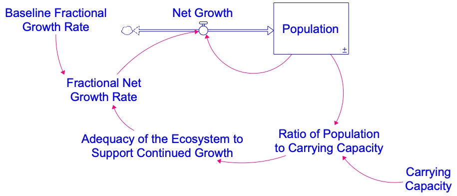
Before you build this model, let’s notice a few important features. First, compare this model to the simple population you built earlier. Can you see that the S-shaped growth model includes all the features of the simpler model, but that it also has some additional features to account for the role of carrying capacity? This illustrates an important principle in system dynamics modeling: We can model more complex systems by using a simpler related system as a starting point and thinking about what additional feedback structure is needed to model the more complex problem (Hines, 2003).
Let’s discuss each of the features in the S-shaped Growth model. Then you will build the model and explore its behavior over time.
- Population stock, Net Growth, and Fractional Net Growth Rate: These three model variable have the exact same meaning and as in the simple population model with a biflow. In addition, the equation for the Net Growth is the same as before: Net Growth = Fractional Net Growth Rate * Population.
- Baseline Fractional Growth Rate: This variable stands for the fractional net growth rate of the Population whenever there are abundant resources on which to live. This variable is used in the equation for calculating the Fractional Net Growth Rate. Because it’s a fractional growth rate, it’s units are fraction/year, dimensionless/year or 1/year. These units are interchangeable.
- Carrying Capacity: This is the population size that the ecosystem can sustain for the long term. Hence, its units are the same units as the stock.
- Ratio of Population to Carrying Capacity As the name implies, this is calculated as the ratio of the Population to the Carrying capacity. This Ratio is less than 1 when the current Population size is less than the Carrying Capacity. In this case, the Population still has “room to grow” in the ecosystem. However, as the Population nears the Carrying Capacity, the Ratio of Population to Carrying Capacity will get close to 1. As this happens, the Fractional Net Growth Rate should slow, moving toward a value of zero. Because both the Population and the Carrying Capacity are measured in people units, when we take the ratio, the units cancel out. Hence, this variable has units that are fraction or dimensionless
- Adequacy of the Ecosystem to Support Continued Growth: This variable is calculated as 1 – (Ratio of Population to Carrying Capacity). When the Population is well below the Carrying Capacity (and the Ratio of Population to Carrying Capacity is hence close to zero), the Adequacy of the Ecosystem to Support Continued Growth value will be close to 1. As the Population approaches the Carrying Capacity (and the Ratio of Population to Carrying Capacity hence approaches 1), thus the Adequacy of the Ecosystem to Support Continued Growth will approach zero. Higher Adequacy of the Ecosystem to Support Continued Growth values imply that the Population can grow at a more rapid place. It has units that are dimensionless or a fraction.
- Fractional Net Growth Rate: This represents the actual Fractional Net Growth Rate of the Population, after accounting for the Adequacy of the Ecosystem to Support Growth of the population. It is calculated by multiplying the Baseline Fractional Net Growth rate times the Adequacy of the Ecosystem to Support Continued Growth. This, in effect, scales down the Baseline Fractional Growth Rate, according to how close the Population is to the Carrying Capacity. The units for this variable are fraction/year, dimensionless/year, or 1/year. Again, those units are all equivalent and you should use the form you are comfortable with.
- UN Low Variant, UN Medium Variant, and UN High Variant. These three variables are included in the model and plotted on the BOTG to provide reference modes (benchmark behavior over time) for comparing your output to the three projections provided by the United Nations. These will be created using graphical functions in Stella Architect®. Because each variable shows the UN projections for world population, their units are people in thousands.
Exercises 4.8: Modeling Challenge – Build the S-Shaped Model
Build the S-shaped model shown here. Note that, along with the Simulated Population curve from the S-shaped model, the BOTG also shows the three UN projections (i.e. Low, Medium, and High Variants). These curves are called reference modes because they display “reference” behavior over time that we want to check our model against. Using reference modes is a common practice among system modelers. Such curves provide a convenient way to compare your model’s output to known historical data or to accepted future projections to see how well the model matches the behavior of those reference modes. We’ll use those reference modes to explore how well the S-shaped growth model can mimic the UN projections.
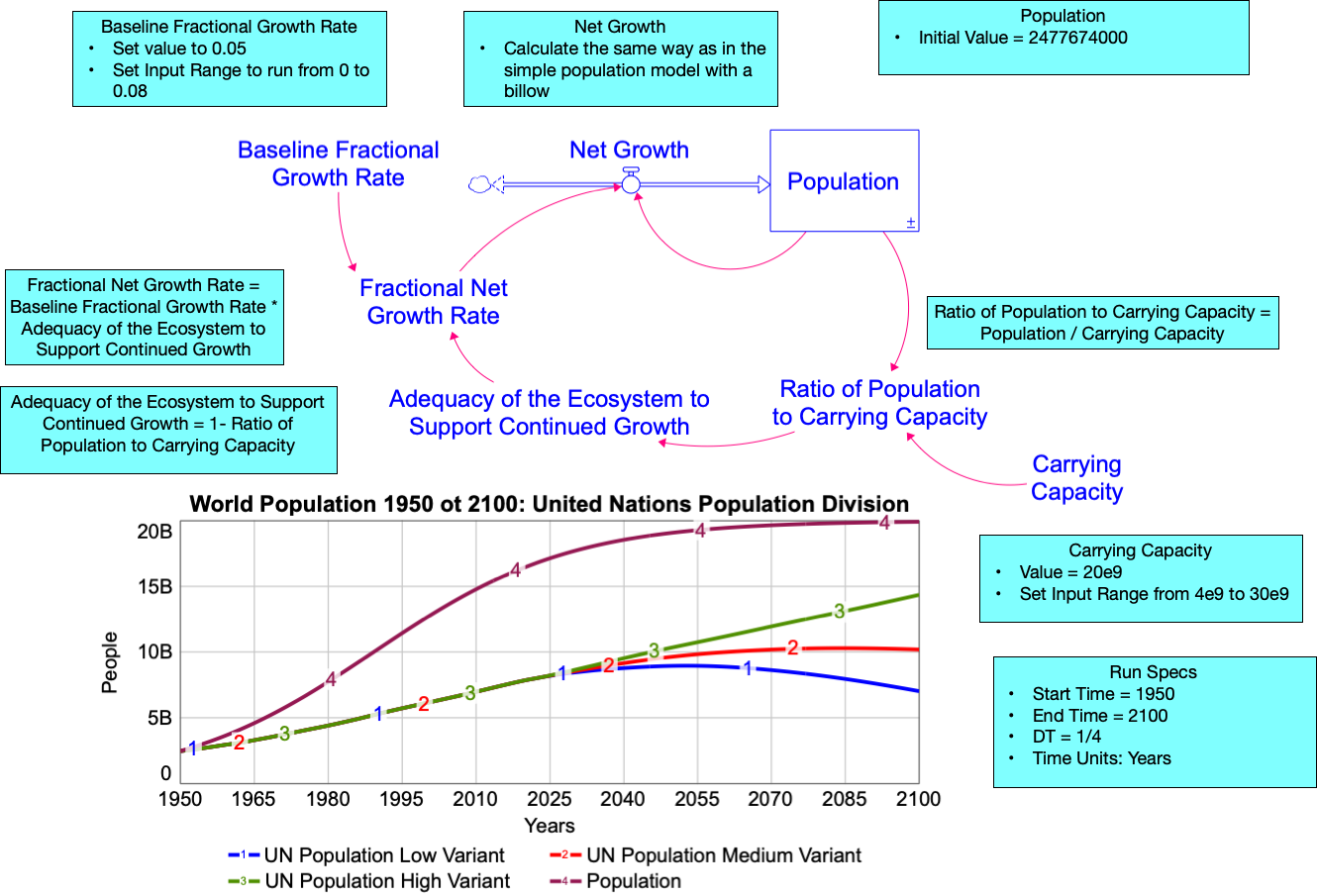
- Label the polarities of the red causal links and the flow (assuming the fractional net growth rate is positive). Also identify and label any feedback loops with circular R1, B1, R2, B2, etc. notation and with descriptive names. Use 14 pt font throughout.
- Specify the variables in each feedback loop so that the entire loop is highlighted when you pass your cursor of the circular loop identifier.
- Run the model with the indicated values and make sure your BOTG exactly matches what you see above.
Exercises 4.9: Modeling Challenge – Does the S-Shaped Model fit the U.N. Projections?
- Adjust the Baseline Fractional Growth Rate and Carrying Capacity to try and match the three variants in the World Population BOTG. Note that each curve may require a different combination of these two variables. Fill out this table:
| Curve on the U.N. Graph | Baseline Fractional Growth Rate | Carrying Capacity | Issues with how well (or not) your model matches the U.N. model. Be as descriptive as possible. |
| Low Variant | |||
| Medium Variant | |||
| High Variant |
- Examine the UN variants from the UN World Population model. Based on the shapes of the chosen curves, identify the range of years when balancing feedback appears to dominate the behavior of the UN projections and the range of years when reinforcing feedback dominates the behavior. If there are time periods when you cannot say for sure what types of behavior dominate the system, identify those. Fill out the table below.
| Scenario | Type of Feedback | Years Over Which it Dominates |
| Low Variant | Balancing | |
| Reinforcing | ||
| Cannot Tell | ||
| Medium Variant | Balancing | |
| Reinforcing | ||
| Cannot Tell | ||
| High Variant | Balancing | |
| Reinforcing | ||
| Cannot Tell |
- Based on these results, when the Carrying Capacity is the largest, what effect does this have on the length of time that reinforcing feedback dominates the system? What about when the Baseline Fractional Net Growth Rate is largest? Explain why this is so.
- Draw a CLD for the S-shaped system, and identifying the feedback loops. See if you can “tell the system story” about how the feedback in the CLD drives the pattern of behavior you see in the BOTG.
4.5.2. Applying S-Shaped Model Structure in Other Contexts
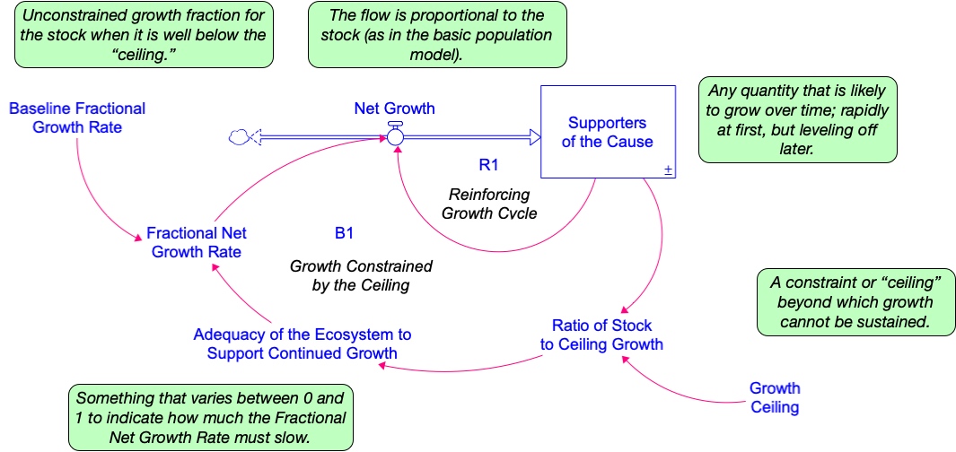
The system structure that gives rise to the S-shaped behavior over time can be used to explain many different types of phenomena that the growth of a population under the constraint of a carrying capacity. In order to see this, look at Figure 4.9, which shows the general stock and flow structure behind the S-Shaped behavior over time, but this time with the variable names in the model changed to be more generic. The text boxes beside several of the variables describe the physical role of each variable in a way that is not directly dependent on the context of a population that depends on an ecosystem for survival.
This kind of system structure has two feedback loops: A reinforcing feedback loop that dominates the system as long as the value of the stock is well below its Growth Ceiling. Under such conditions, the Stock will grow exponentially. However, as the Stock grows, it eventually approaches the Growth Ceiling and triggers mechanisms that begin to dampen its growth. These mechanisms are not specified in the diagram (it depends on the specific context). Their collective action, however, is represented in the variable Adequacy of the System to Support Continued Growth – a value that approaches zero as the Stock approaches the Growth Ceiling. In this formulation, the Adequacy is multiplied times the Baseline Fractional Net Growth Rate to determine the actual Fractional Net Growth Rate. This effectively drives the Fractional Net Growth towards zero, leveling off the growth trajectory of the Stock.
The next Team Modeling Activity gives you practice applying the S-shaped stock and flow structure to some new contexts.
Exercises 4.10: Team Modeling Activity – Apply the S-Shaped Model to Other Contexts
You will work in teams of 3-5 people during class time in order to complete the challenge. Your instructor will be present to help if your team gets stuck, but not to give you the answers!
Each numbered item below describes a situation exhibiting S-shaped behavior over time. For each case, adapt the S-shaped model to match that situation. For each problem, do the following:
- Sketch out on the wall (using a whiteboard or poster paper) the stock and flow structure for the indicated system.
- Give names to the stocks and flows that correspond to the context.
- Write on the wall the equations for each flow, and the starting values for the stocks.
- Then build the model in Stella®. In some cases, you may need to eliminate one of the flows or add an additional stock and corresponding flows.
Once you build each model, draw a simple Causal Loop Diagram (without drawing stocks and flows) showing the feedback loops in the system. Be ready to use your CLD to tell the story about how the feedback structure drives the behavior of the system. You could use the same model you built and simply change the variable names, numeric values, and units to match that particular case.
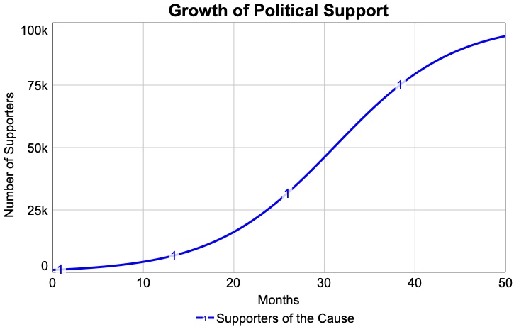
- The number of People Supporting a Political Cause increases exponentially, so that, as the cause grows in popularity, even more people “get on the bandwagon” of support. This continues up to a point. Suppose that only a certain number of people in the population (call it the Potential Support Base) could conceivably support the cause. As the number of actual supporters approaches the size of the potential support base, the growth in support for the cause will slow and eventually stagnate. Assume that the number of supporters is 1000 people and that the Potential Support Base is 100,000 people. Also assume that, because of a highly effective ad campaign, every month the People Supporting the Cause increases by a net rate of 15%. How long will it take for the People Supporting the Cause to reach 20,000? 50,000? 75,000? When you build your model, you should get a BOTG that matches the graph below.
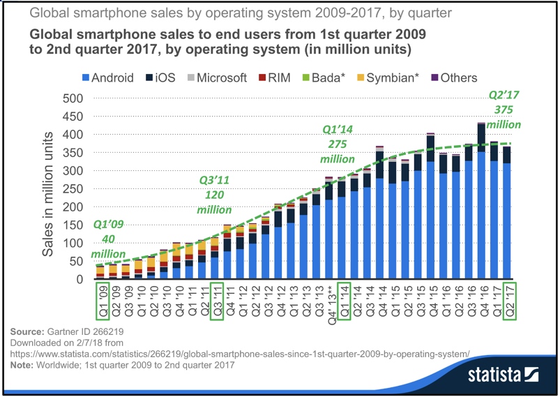
- Whenever an innovative new product is introduced into a market its sales can grow exponentially for many years until the market begins to approach “saturation” (the point at which the sales growth slows, and no new populations are left for the product to “penetrate.” For example, look at the BOTG of smartphone sales from 2009 through the 2nd quarter of 2017. Notice how, apart from some random fluctuations, this graph shows a roughly S-shaped curve, as shown by the dashed line sketched onto the graph. Adapt the S-shaped growth model to represent this situation. Assign units and physical descriptions to each of the variables. See if you can “tune” the model to match the behavior you see in this graph. Do this by matching as closely the four sales figures that are shown in green on the graph.
3. Advanced challenge: Consider the smartphone sales example from the previous question. The BOTG suggests that smartphone sales are leveling off. That’s because the Growth Ceiling in Figure 4.9 is assumed to be a fixed constant. In reality, that is not how things actually work. When a smartphone manufacturer develops their product, they continually work to “expand the market” by giving their phone features that will appeal to a broader audience. For example, they develop a breakthrough manufacturing process that dramatically decreases the price of their phones. Or they might introduce a much more powerful and versatile camera on the phone. If they are successful, the number of potential buyers would dramatically increase, as more people are attracted to the phone (and as existing customers upgrade to the new model). See if you can adapt the model you developed in the previous exercise so that the number of potential smartphone buyers doubles in the 40th quarter of the simulation. You can do this by adding a multiplier variable whose value is 1 for the 1st 40 quarters and then shifts to a value of 2 for the rest of the simulation. This can be done by using a step function. Use that new variable as a multiplier to calculate the number of potential buyers. Run the simulation for twice as long and see what happens.
4.6. Reflections on the Journey so Far – How Structure Creates Behavior
When you built the S-shaped growth model, you created a system story to explain how the feedback structure in this system creates the S-shaped growth behavior over time growth curve. Such stories are possible because of the simple truth that structure determines behavior. By this we mean that the feedback structure in a system is the most important determinant of how that system will behave over time.
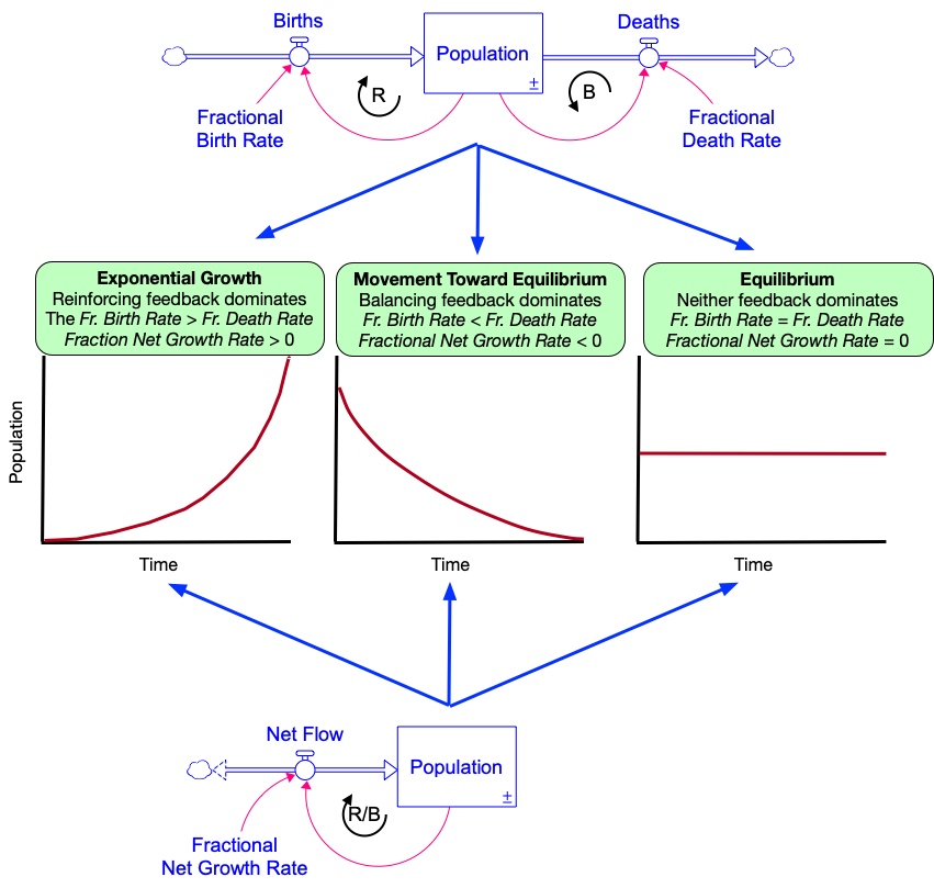
For example, consider the original population model. The original model with separate birth and death flows models includes two feedback loops: one balancing loop and one reinforcing loop. As you learned earlier, reinforcing feedback leads to growth, and balancing feedback leads to movement toward equilibrium. Hence, a system like the simple population model can exhibit only two types of behavior[1], depending on which of these two feedback loops dominate.
- Exponential growth – This occurs when the reinforcing feedback in Figure 4.9 dominates the behavior of the system — and that happens when the Fractional Birth Rate exceeds the Fractional Death Rate, or in the net flow model, when the Fractional Net Growth Rate is positive.
- Movement toward equilibrium – This occurs when the balancing feedback in Figure 4.9 dominates the system — and that happens when the Fractional Birth Rate is less than the Fractional Death Rate, or in the net flow model, when the Fractional Net Growth Rate is negative.
- Equilibrium – This will occur in two situations:
- When there are no people present. In that case, there are not births or deaths, and the population will remain at zero.
- When both feedback loops exhibit equal influence on the system. This happens in the original model when the Fractional Birth Rate is equal to the Fractional Death Rate, or in the net flow model, when the Fractional Net Growth Rate is zero.
Since the Fractional Birth and Death Rates (or the Net Growth Rate) are fixed quantities in this model, the relative influence of each of the feedback loops in this system does not change over time. That is, the system exhibits only one of the above three behaviors for the entire period we simulate. See Figure 4.10.
The S-shaped growth system also has only two feedback loops. Why is it that this model produces more complex behavior than we see with the simple population models? The answer is that the relative influence of the two feedback loops in the S-shaped growth model changes over time. That is, neither feedback loop dominates all the time! Early on, the reinforcing feedback dominates the system. Later, the balancing feedback dominates the system.
You can see this shift in loop dominance by examining the BOTG created by the S-shaped model, as shown in Figure 4.11. Notice that, early on, the graph exhibits exponential growth ― the graphical signature of reinforcing feedback! Then later on, as the Population size approaches the system’s Carrying Capacity, the BOTG exhibits the kind of goal-seeking behavior that comes from a balancing feedback loop.
To be sure, both feedback loops are work during the entire simulation. However, their relative influence on the behavior of the Population stock varies over time.
But why does this shift actually happen? What is it about the real-life system that causes this? Common sense would suggest that, early on, the population has abundant resources to support growth. Hence, exponential growth is the logical result. However, as the Population grows, it gets closer to the Carrying Capacity of the ecosystem. This means that there are not as many resources to go around. Fewer people are born; fewer can survive with the existing resources. Hence, Population growth slows, and eventually levels off at zero growth, as in Figure 4.11.
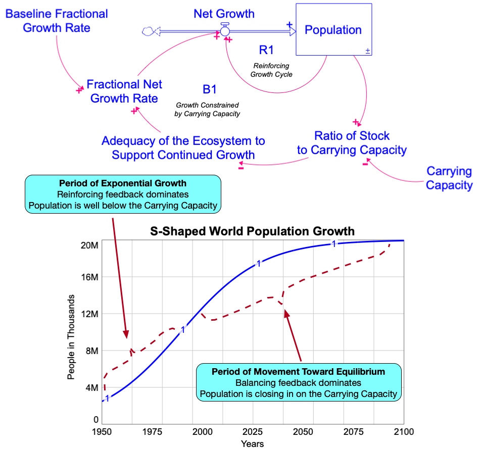
The point of all of this discussion is to illustrate how an analysis of the feedback structure in a system can give us insights into why it behaves in the ways we see in a simulation or a real-life BOTG of historical trends.
Of course, real life systems can exhibit even more complex behavior than S-shaped growth. When this happens, it means that the underlying system has a more complex feedback structure than what we’ve seen so far.
Consider the United Nations’s low variant curve in the World Population BOTG graph shown earlier. This early part of this curve mimics the exponential growth of both the high variant and medium variant curves. What causes the low variant curve to decline instead of leveling off toward the global carrying capacity? In a later section you will explore this question by examining a system structure that can mimic this behavior quite nicely – the overshoot and collapse structure.
4.7. Making Your Model Available to Others: Building a User Interface
One of the best ways to explore a system dynamics model is create a user interface that allows you and others to experiment with the variables in model and see how they the affect the behavior of the system. This kind of experimentation gives you insights into how the model works. If the model is reasonably valid (i.e. “useful” in the sense that G.E.P. Box meant), then experimenting with it can help you understand how the real-life system works. This can be immensely helpful to anyone who has to make decisions that impact the system.
Models that are used in this way are called virtual worlds or microworlds[2] (Sterman, 2006). These models are used as a rough approximation to the system we wish to influence.
You may realize that you have already played with a microworld. In the Kaibab challenge you interacted with a user interface for a system dynamics model of the Kaibab ecosystem. The figure below shows that interface. This particular interface allowed you to adjust variables in the model corresponding to real-life decisions made back in 1907. You made adjustments and watched them play out in the BOTG. You didn’t have access to the underlying stock and flow model. At that time in the course, you would probably have been overwhelmed by the all the stocks flows, and causal connections in the model. Besides, we wanted your experience to feel as “real” as possible. Since the real-life decision makers back in 1907 didn’t have access to the model structure, neither did you!
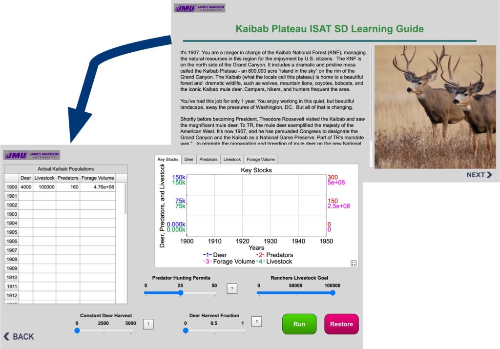
An important skill of any system dynamics modeler is to be able to create useful interfaces that allow others to experiment with the system and learn about the connections between actions and their outcomes. Most system dynamics software packages allow you to build user interfaces. Stella Architect® has an excellent utility for this.
In addition to allowing a user to experiment with the model, a good user interface can also educate them on why the system behaves the way it does. This is done by including in the interface a system story that logically unfolds the feedback structure in the system and explains how that structure creates the behavior over time that we see in the graphical output.
In the next Modeling Challenge you will build a user interface of the S-shaped growth model. Your instructor will guide you through this process. Once you finish, you will have your own microworld that you and others can use to run experiments, follow the system story, and better understand the dynamics of this system.
Exercises 4.11: Modeling Challenge – Build a User Interface for the S-Shaped Growth Model
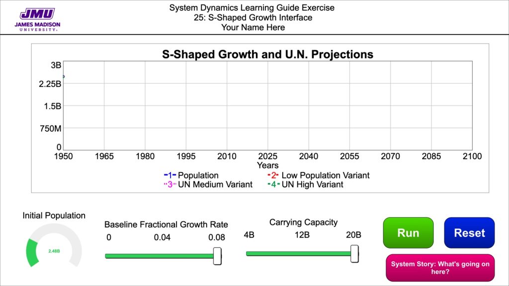
Your interface will allow users to explore how the system behaves when: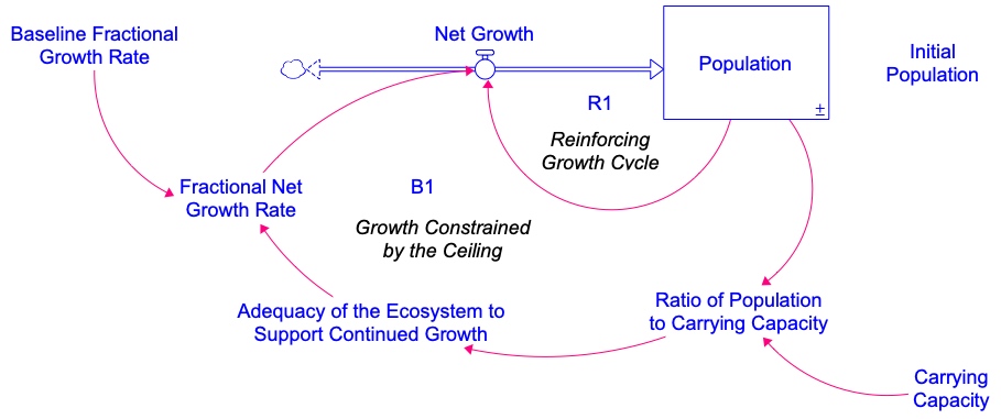
- The Carrying Capacity varies over time
- The Baseline Fractional Growth Rate varies over time.
- The Population starts out higher than the Carrying Capacity of the system.
It will also include an interactive system story that explains to the user how the feedback structure in the system creates the S-shaped BOT.
When you finish, the main menu on your interface should look the image below. Important: Make sure your model has been corrected for any errors from you earlier effort.
Once you finish the interface, run the model and see if you can find a fixed value for the Baseline Fractional Net Growth Rate and then dynamically change the Carrying Capacity during the run to more closely match the Low Variant UN projection. Be ready to discuss what you found. You can go an online version of the model by clicking here.
4.8. Overshoot and Collapse – Non-Renewable Resources and Eroding Carrying Capacity
The UN’s low variant curve corresponds to the situation in which the world population overshoots the earth’s carrying capacity and subsequently drops back to a sustainable level. This decline might be caused by conflict over resources, disease, or other factors. This kind of decline is possible if one (or both) of the following two situations exists:
- There is a delay in information so that the humans don’t realize that the global population is approaching (or has maybe even exceeded) the global carrying capacity. After all, no one really knows for sure what the earth’s carrying capacity is. Besides, even if someone knew what size of population could be supported on earth, how would that be communicated to everyone on the planet? Why should anyone believe it? Who would have the political authority to enforce lower birth rates to make sure we didn’t overshoot the carrying capacity? Would it even be right for someone to have that kind of authority? All of these issues are at least part of the reason that humans could exceed the global carrying capacity and not realize it for some time, maybe for a generation or more.
- The carrying capacity of the planet is not constant. It could increase over time because of technological advances, such as more productive agricultural practices. On the other hand, the global carrying capacity could decrease over time drop as things like pollution and deforestation degrade the capacity of the global ecosystem to support human life. Large scale air pollution, water pollution, and the challenge of human-driven climate change are known realities, and their effect on the earth’s carrying capacity is not fully understood.
These two possibilities suggest an approach to modeling the kind of overshoot and decline (or overshoot and collapse) behavior that we see in the UN’s low variant curve for human population. We can do this by adding a stock and flow structure that shows how the earth’s carrying capacity depends on some natural resources whose status changes over time. For example, if the world population depends on some non-renewable resource for survival, the degradation or consumption of that resource would jeopardize lives. Oil and other fossil fuels are resources that exist in finite quantities that are not expected to change appreciably over millions of years. And yet, much of modern society is based on the availability of those resources. What happens when or if those resources are depleted?
Figure 4.13 shows a stock and flow diagram corresponding to this kind of situation. We call this model an Overshoot and Collapse Model because it identifies a generic system structure by which a population might overshoot its carrying capacity and subsequently collapse to a much smaller size. Notice that this diagram looks very similar to the S-shaped growth model, but with some important changes. The next two Modeling Challenges give you a chance to explore the structure of this model and to build a running simulator.
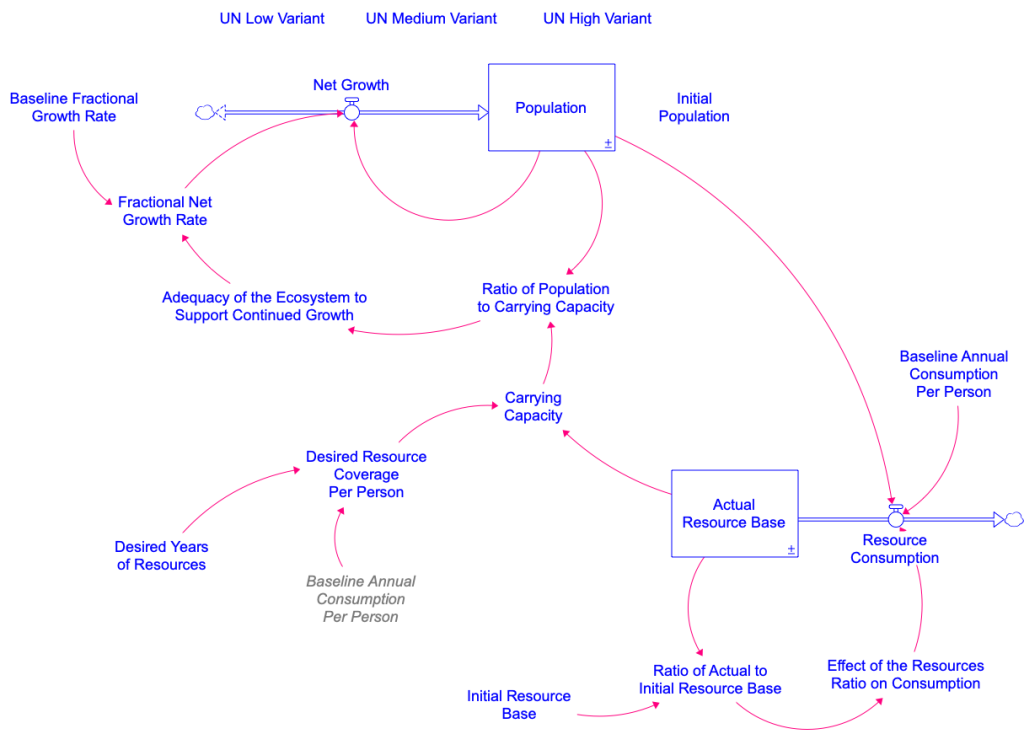
The explanation of the variables in Figure 4.13 follow:
- Population, Net growth, Fractional Net Growth Rate, Baseline Fractional Growth Rate, and Adequacy of the Ecosystem to Support Continued Growth ― See the discussion on the S-shaped growth model and use the same model setup, values, and equations for these variables, as outlined in the Modeling Challenge: Build the S-shaped model with one exception. The Baseline Fractional Growth Rate should be set to 0.05. Note that, unlike in the S-shaped model, the Carrying Capacity in the overshoot and collapse model is no longer a constant value. Details on this variable are given below.
- Ratio of Population to Carrying Capacity: This has the same physical interpretation and units as in the original S-shaped growth model. However, in this model, the Carrying Capacity will decline as the Actual Resource Base is consumed by the Population. Hence, the Carrying Capacity may reach zero if all the resources are consumed. To avoid dividing by zero in this ratio, we use the built-in function that prevents division by zero. The built-in is simply a double division in the equation. Carrying Capacity is now Population//Carrying Capacity.
- Desired Years of Resources: The global average lifespan of humans (71 years in 2021) (Saloni, et al., 2023). This is used to calculate the Desired Years of Consumption (described shortly). This modeling structure assumes that Carrying Capacity is determined by the amount of resources needed to last for the average human lifetime. Anything less than that will cause widespread awareness of resource shortages, leading to lower consumption rates (this might be an optimistic assumption so feel free to experiment with different values for this constant).
- Desired Years of Consumption: This variable captures the concept of whether enough resources are available to continue operating as we have in the past. We are being explicit about consuming non-renewable resources, but the consequences of running out are in the future, and our behavior may not be changed until the scarcity becomes evident in our lifetime.
- Baseline Annual Consumption per Person: The amount of resources consumed per person per year whenever resources are plentiful. This variable also has a ghost version in the model. A ghost is an exact copy of the original variable. We use ghosts to avoid drawing long causal links that cross over other parts of the diagram. This is purely for cosmetic purposes to make the diagram easier to read. In the diagram, we’ve used the convention of showing it with an italic font and different colors. Measured in units of Resources/(People * years).
- Actual Resource Base: The stock of nonrenewable resources that the population depends on for survival. Set the initial value of this stock to be equal to the Initial Resource Base (next variable). Measured in units of Resources.
- Initial Resource Base: An exogenous variable used to set the starting value for the Actual Resource Base. Measured in units of Resources.
- Resource Consumption: The consumption of the resource by the human Population. The amount of resources consumed per year is determined by the number of people in the Population, the Baseline Annual Consumption per Person, and the Effect of the Resources Ratio on Consumption (explained below). Units are Resources/Years.
- Ratio of Actual to Initial Resource Base: The comparison of the Actual Resource Base to the Initial Resource Base. This comparison measures the fraction of the Actual Resource Base to the Initial Resource Base. A value close to 1 indicates that resources are plentiful and near their original condition. A value close or approaching 0 indicates that resources are becoming depleted. Measured in units that are dimensionless.
- Effect of the Resources Ratio on Consumption: This is a nonlinear function that captures the idea that people will continue to consume resources at a regular rate until the resources fall below 50 percent. At this point, resources are more difficult to extract and less is consumed. The nonlinear function falls to zero when no resources are left as it is physically impossible to consume non-renewable resources once they are gone. The exercise below will provide you with information to build this nonlinear function. The units are dimensionless.
- Carrying Capacity: Same as before – the number of people that the system can support. In this case, it is calculated as the number of people that the Actual Resource Base can support, assuming that people consume the resource at the annual rate defined by the Baseline Annual Consumption per Person, and assuming that enough resources are needed to sustain the human population for one lifetime. Units are People.
- UN Low Variant, UN Medium Variant, and UN High Variant: These are the same graphical function variables used in the S-shaped model. You can simply copy those variables from that model and paste them into this model. However, do not copy and paste these variables until you’ve set the model settings to their proper values.
Exercises 4.12: Modeling Challenge – Understand the Overshoot and Collapse Model Structure
Refer to the diagram below and the above explanation of the model variables to complete the following tasks.
- Draw a line around that part of the diagram in Figure 4.13 that corresponds to the S-shaped growth model we covered earlier.
- In this overshoot and collapse model, the Carrying Capacity is now an endogenous variable (meaning that it is part of a feedback loop and its value can vary over time, as represented by the causal links pointing into it in the diagram). Why does this makes sense?
- Given the above description of the Desired Years of Consumption in this model, which of the following is the most logical way to calculate the Desired Years of Consumption?
- Baseline Annual Consumption per Person / Desired Years of Resources
- Desired Years of Resources / Baseline Annual Consumption per Person
- Baseline Annual Consumption per Person * Desired Years of Resources
- Baseline Annual Consumption per Person – Desired Years of Resources
- Baseline Annual Consumption per Person + Desired Years of Resources
- Desired Years of Resources – Baseline Annual Consumption per Person
- Desired Years of Resources + Baseline Annual Consumption per Person
- Some other equation (specify):
- This value is not calculated with a formula. It’s a fixed value set at the beginning of the simulation.
- Given the description of the Resource Consumption outflow, which of the following is the most logical way to calculate this variable?
- This value is not calculated. It is a fixed value that is set at the beginning of the simulation.
- Baseline Annual Consumption per Person * Effect of the Resources Ratio on Consumption * Population
- Population * Effect of the Resources Ratio on Consumption / Baseline Annual Consumption per Person
- (Population – Baseline Annual per Person) * Effect of the Resources Ratio on Consumption
- (Population + Baseline Annual per Person) * Effect of the Resources Ratio on Consumption
- (Population – Baseline Annual per Person) / Effect of the Resources Ratio on Consumption
- (Population + Baseline Annual per Person) / Effect of the Resources Ratio on Consumption
- Some other equation (specify):
- What is the polarity (+ or -) of each of the two links that point into the Carrying Capacity? Explain your reasoning for each polarity.
- Given the description of the Effect of the Resource Ratio on Consumption and its role in the model diagram, what do you think should happen to this Consumption Rate as the Ratio of Actual to Initial Resource Base declines? Explain your answer.
- It should remain unchanged
- It should get smaller
- It should get larger
- There is no way to tell.
Exercises 4.13: Modeling Challenge – Build the Overshoot and Collapse Model with an Interface
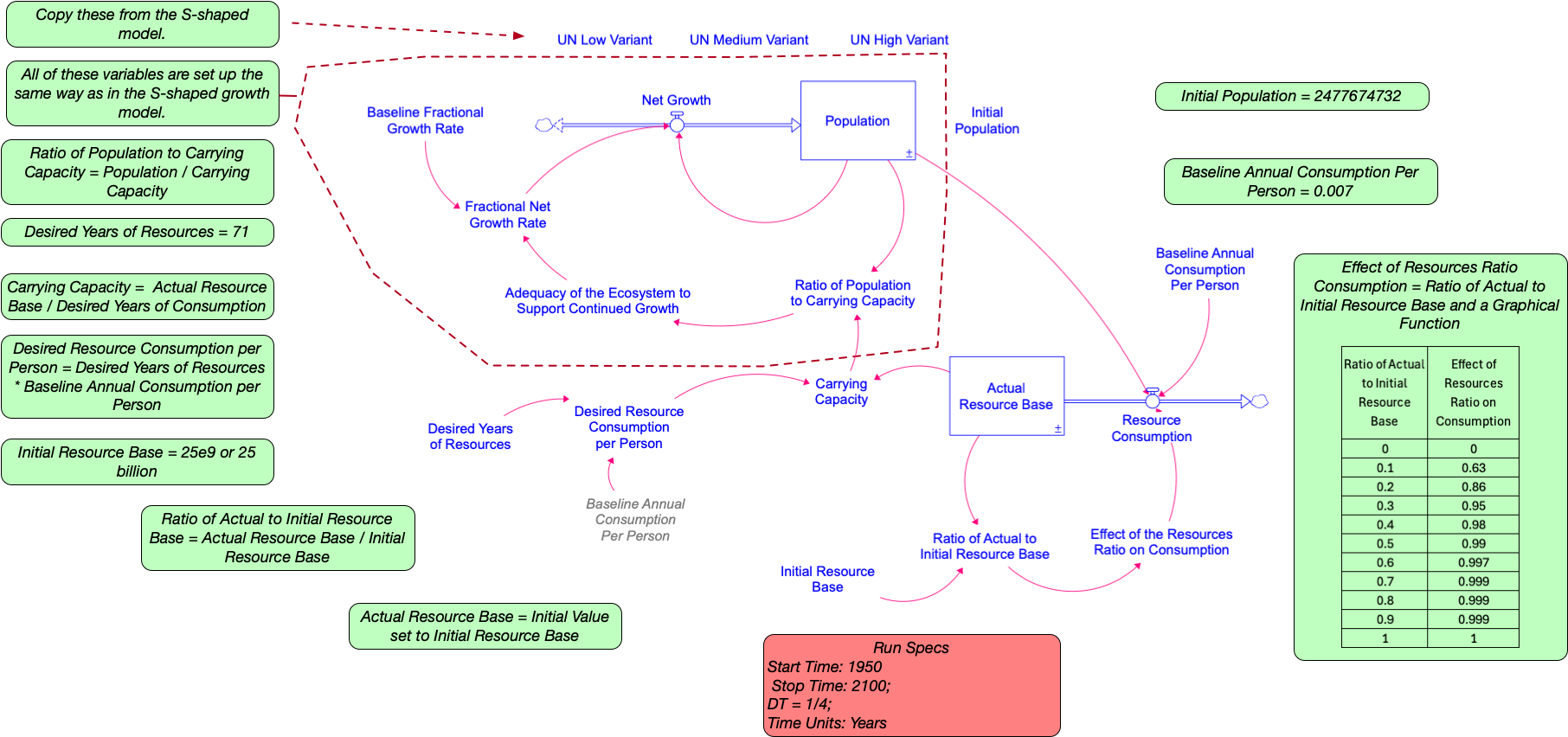

- Based on the insights you gained from the previous Modeling Challenge, plus what you’ve learned working with the S-shaped growth model, build the overshoot and collapse model.
- Make sure your model gives you the exact same BOTG that you see above.
- Attach +/- polarities to all causal links. In addition, identify and label all the feedback loops (there are four of them!). Use Stella® to identify the variables involved in each feedback loop, so that, when you place your cursor over the circular R or B labels, the variables involved in the loop are highlighted.
- Create a user interface in Stella which looks like the following.
- Draw a CLD (without the stock and flow symbols) for the system. You can do this by hand or with the software.
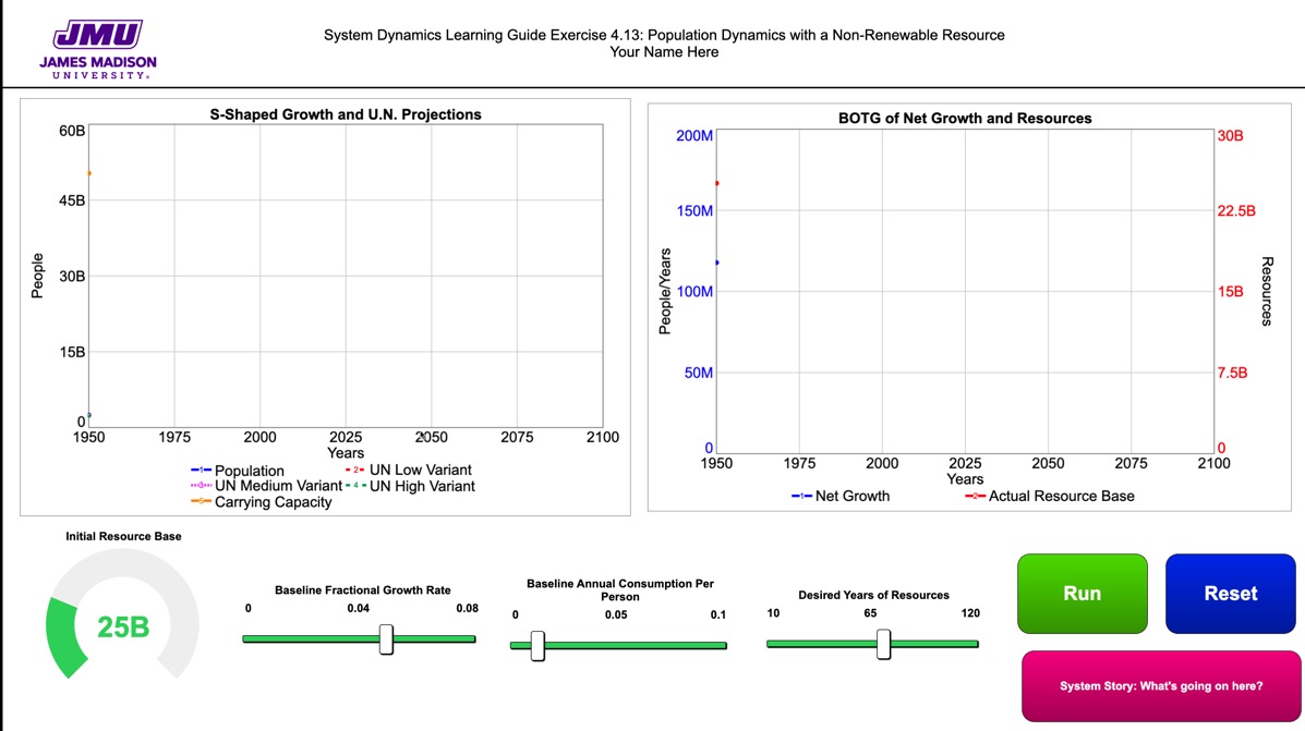
The system story will have the following three pages. When you create the pages, make sure you show the link polarities, as well as the circular R/B loop identifiers and descriptive names for each of the feedback loops. Add callout text to each page of the story to explain how the feedback shown on that page affects the system behavior. On pages 2 and 3, make sure you explain how the new feedback on that page changes the behavior from the previous page. Note that this story does not show all of the variables in the model. This is a common practice: to show only as much detail as is needed to tell your story.
Once you finish your model and interface, check it against this online version to make sure your interface works the same way and that the simulation results and BOTG graphs match up.
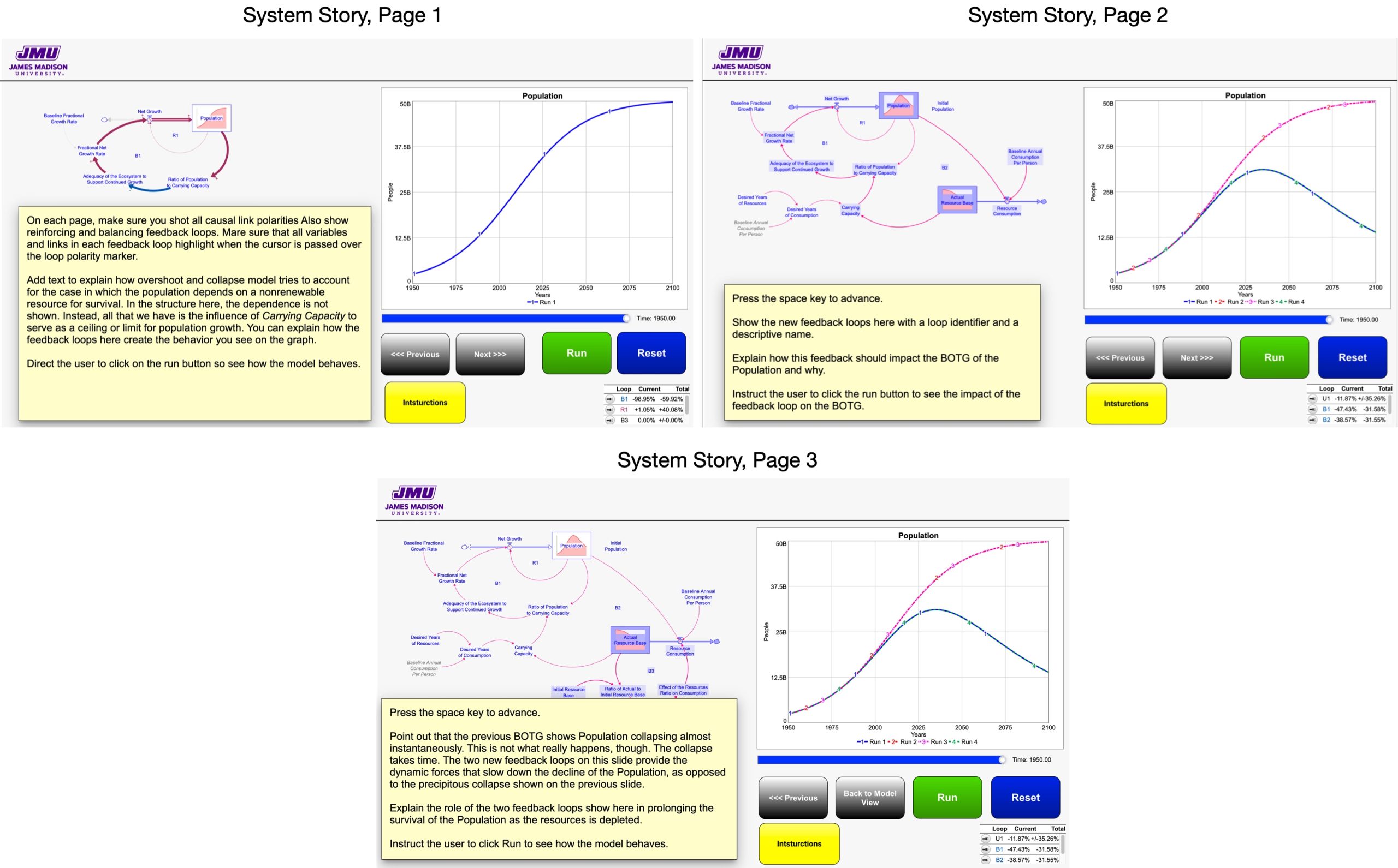
Exercise 4.14: Modeling Challenge – Apply the Overshoot and Collapse to the United Nations Projections
- Perform experiments with your overshoot and collapse model by adjusting each of the following variables in turn (i.e. adjust only that variable, leaving the others at their original values). Observe how the BOTG changes with those adjustments. Then for each variable briefly describe how changing it affects the behavior over time of the two stocks.
- Desired Years of Resources
- Baseline Annual Consumption Per Person
- Baseline Fractional Growth Rate
- Initial value for the Actual Resource Base stock. Do this by changing the value of the Initial Resource Base.
- Which feedback loops in the overshoot and collapse model do you think work in such a way to enable the Population to grow for too long so that it overshoots the carrying capacity? Explain.
- Identify combinations of the above variables that result in a BOTG that matches each of the UN’s Low, Medium, and High variant curves. Fill out this table.
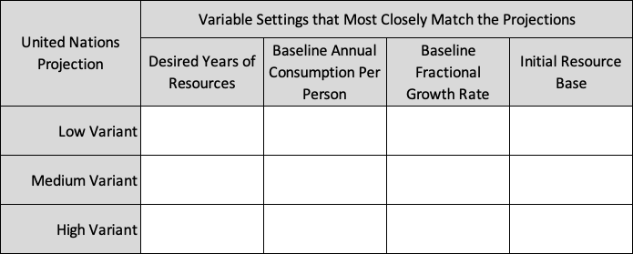
4.9. Population Growth with Renewable Resources: Achieving Sustainability
In the previous overshoot and collapse model, the Population exceeded the carrying capacity of the system partly because that carrying capacity depended on a nonrenewable resource that was consumed by the Population. The fact that the Actual resource stock in that model has only an outflow means that the resources will never be replenished. They will only decline. As a result, the carrying capacity in the system erodes over time as the resource base is consumed, and the population eventually collapses.
However, it may be that the resources are renewable. Critical resources such as water or food can be replenished with the seasons of the year through agriculture and other methods. The next Action Item gives you an opportunity to enhance the original overshoot and collapse model by adding an inflow into the Resource stock, making it a renewable resource.
Exercises 4.15: Modeling Challenge – Population Growth with a Renewable Resource
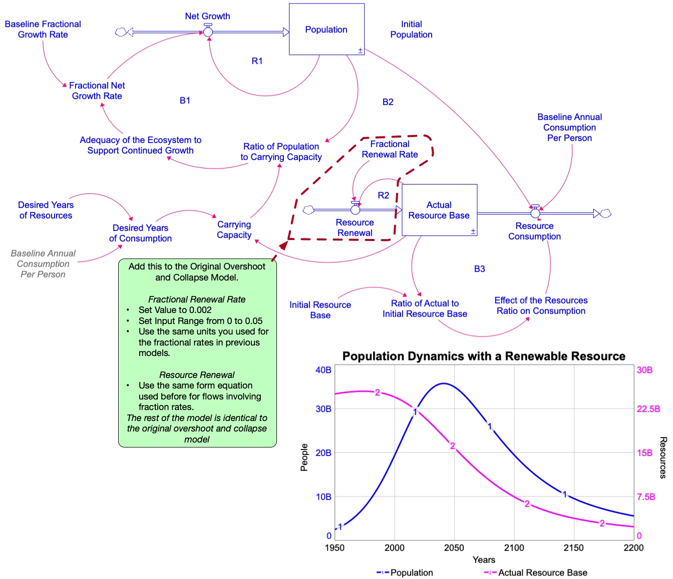
- What are the units for the Fractional Renewal Rate? For the Resource Renewal inflow?
- What is the proper equation for calculating the Resource Renewal inflow?
- Build this model, beginning with the overshoot and collapse model you built earlier.
- Identify combinations of the Desired Years of Resources, Baseline Annual Consumption per Person, Baseline Fractional Growth rate, and Initial Resource Base starting value that result in a BOTG that matches each of the UN’s Low, Medium, and High variant curves. Fill out this table.

5. Now compare the model variable values you used to mimic each of the three variants. What do these differences in those values suggest about how the practical conditions under which the human population might end up following each of the UN’s curves?
4.10. Oscillation: A Predator-Prey Case Study
4.10.1. Introduction to Oscillatory Behavior
Up to this point in your modeling journey, you have modeled the basic dynamics that dictate the future of a population, be it a population of humans, animals, or plants. You have also learned how the feedback structure affecting population dynamics can serve as a framework for modeling system behavior from a variety of problems that, on the surface, seem far afield from the problem of population growth.
That’s part of the beauty of using system dynamics as a lens for looking at the world. The dynamics affecting the support of political cause or the sale of smartphones may appear on one level to be quite different from those that affect the growth of a population. However, through the lens of system dynamics, we find that the underlying feedback structure of these seemingly different phenomena can explain the behavior of a widely varying collection of real-life phenomena.
We now turn our attention to another type of behavior over time that is common in nature and human activities: oscillatory behavior. We will use the dynamics related to the predator-prey relationship as a case study to help us explore some ways this type of behavior can arise. In particular, we will return to the Kaibab Plateau to model the dynamic relationship between the Kaibab mule deer population and the population of predators that depend on the mule deer for food.
An important theme to remember as we examine the dynamics of oscillatory behavior is the following.
Feedback and Oscillatory Behavior
Oscillatory behavior can be created by the influence of a major balancing feedback loop.
A second-order feedback loop contains two stocks.
A major balancing feedback loop is capable of generating sustained oscillations.
A minor feedback loop contains only one stock and is not capable of generating an oscillation.
A major and minor feedback loop are capable of generating dampened oscillations.
In predator-prey systems, the stocks of predators and their prey often oscillate around equilibria levels over time (see Figure 4.14). Initially, both populations exhibit a steady state (constant) pattern at two different equilibrium levels: one equilibrium for the prey population, and another for the predator population. The equilibrium levels are those population sizes at which the predators and prey co-exist in a steady-state balance. The predators kill just enough prey to maintain their population size, and the prey would grow at a rate to offset the deaths through predation (and other natural causes).
Notice, however, that about ⅓ of the way into the simulation, something happens to “kick” the system out of equilibrium. At this point, both populations start to oscillate around their respective equilibria. This is how such systems work. If, for any reason, either population moves away from its equilibrium point, both populations will begin to oscillate…sometimes indefinitely, but often for a limited time until the system settles back into equilibrium (as seen in Figure 4.14).
Why does this oscillation happen? Imagine, for example, that a disease strikes the prey population, so that many prey die. You can see this in Figure 4.14 by the sharp drop in the prey population ⅓ of the way into the BOTG. This drop in the prey population creates a food shortage for the predators, so that a predator population can no longer be supported at the equilibrium size; the predators will decline in numbers. This allows the prey population to rebound (since there are fewer predators in the system to hunt and kill prey). As the prey population rebounds, the predator population will follow suit as it becomes easier for them to find food. The process can continue for some time as the predator and prey populations “seek out” their respective equilibria.
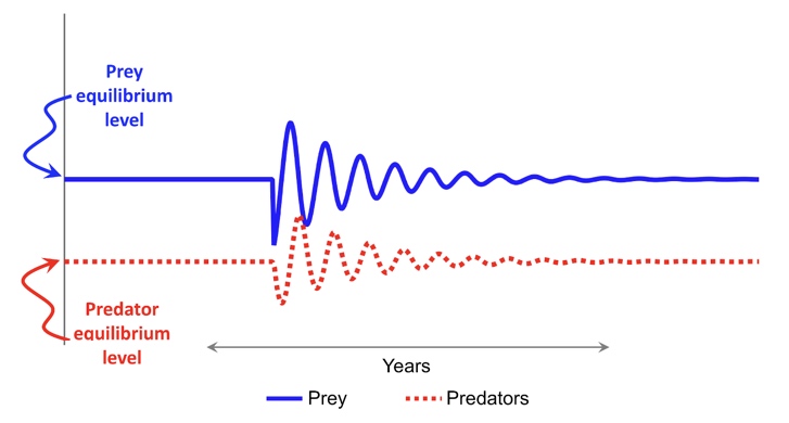
What sort of feedback structure creates the kind of behavior we see in Figure 4.14? There are many different formulations of how the predator-prey system works[3], but all of those formulations involve a feedback structure that is similar to the one shown in Figure 4.15. Let’s examine that figure to see how the structure in this model makes sense for the predator-prey problem.
4.10.2. Telling the Story: How Feedback Creates Oscillations in the Predator-Prey System
To understand how the feedback structure in the Predator-Prey model can create oscillations, we must first understand the role played by each of the five feedback loops in this model.
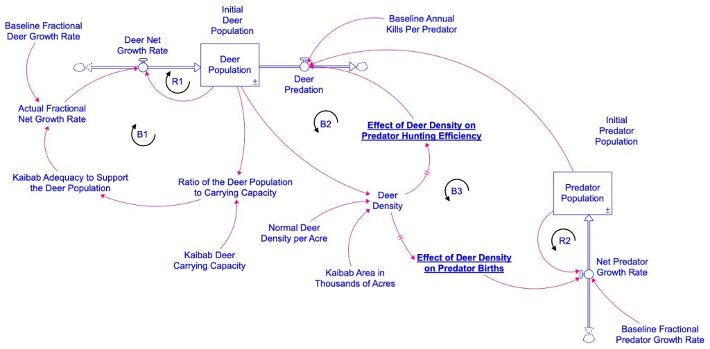
- Loops R1 and B1: S-Shaped Growth Dynamics. The upper left portion of the model corresponds to the usual S-shaped growth structure we have seen several times. That is, one set of dynamics affecting the status of the deer population are those dynamics associated with natural unconstrained growth (R1 loop) and the constrained growth as the deer population approaches the carrying capacity of the system (B1 loop).
- Loop R2: Simple Predator Population Dynamics. The R2 feedback loop represents the force of unconstrained growth on the Predator Population, just as in the simple population model. This kind of growth would be possible in the presence of an infinite food supply. Of course, this is not the case – a reality that is captured in some other feedback loops in the system. The Net Predator Growth Rate is a biflow indicating that negative values will allow the flow to reverse course and flow out of the stock. This captures the concept that predators could die of starvation if there is not enough prey.
- The Dynamics Behind Oscillation: One Major Feedback Loop.
We noted earlier that a major balancing feedback loop (a feedback loop with two stocks) oscillatory behavior is possible. The B3 feedback loop is the major loop and contains a stock for deer and one for predators. The B2 feedback loop is a minor negative loop. The combination of the the B3 and B2 feedback loop generate the dampened oscillation observed in Figure 4.14. You will notice in Figure 4.15 that there is a double hash mark on the causal links running into the Effect of Deer Density on Predator Births and into the Effect of Deer Density on Predator Births. This hash mark is used to indicate delays in the feedback loop. - In this case, there is a delay in the effect of Deer Density on the two Effect variables. By this we mean that minor changes in Deer Density will not result in immediate sizable changes in either Effect variable. Instead, Deer Density must consistently increase (or decrease) for a period of time before it has an appreciable effect. The two bullets below explain how these two feedback loops work and why the indicated delays make sense.
- Loop B2: The role of predation. Feedback loop B2 represents balancing effect of predation to keep the size of the Deer Population from getting too large or too small. Through this feedback loop, a decline in the Deer Population through predation is constrained by the effect of Deer Density on the Effect of Deer Density on Predator Hunting Efficiency. In particular, if there are fewer deer (so that Deer Density decreases), predators will be less efficient in finding deer for food and less deer will die through predation, allowing the Deer Population to rebound. If the Deer Population grows, then Effect of Deer Density on Predator Hunting Efficiency will also increase, leading to more Deer Predation and a subsequent decline in the population. The Effect of Deer Density on Predator Hunting Efficiency is a nonlinear function with a positive slope. The slope flattens out as the Deer Density doubles or declines towards zero. An increased Deer Density indicates an abundance of deer and predators will kill more deer up to a certain point. Predators kill to eat and reducing hunting when satiated. The same logic applies when Deer Density declines. Once Deer Density drops to critical levels, the Effect of Deer Density on Predator Hunting Efficiency is evident; increased hunting activity by predators will be insufficient to compensate for the loss in food supply.
- Loop B3: The mutual interaction between the Deer Population and the Predator Population. This feedback loop represents the dynamics by which changes in the Deer Population and the Predator Population puts in motion forces that generate the oscillation. This loop represents a mutual effect that the Deer and Predator Populations have on one another. As the Deer Population increases, more deer are killed and eaten by Predators, fueling growth in the Predator Population. This in turn leads to over-hunting of deer and a subsequent decline in the Deer Population. Each stock represents a delay as the inflows and outflows are decoupled and take time to react to changes. The B3 feedback loop also contains a nonlinearity captured in the Effect of Deer Density on Predator Births. The slope of this nonlinear function is positive and when Deer Density is one, the Effect of Deer Density on Predator Births will be zero. That is births and deaths are equal and the predator population will not change. When the Deer Density is above one, the Effect of Deer Density on Predator Births will be positive and the Predator Population will grow. When the Deer Density is less than one, the Effect of Deer Density on Predator Births will be negative, meaning that deaths are greater than births, and the Predator Population will decline.
4.10.3. Another Look at the Oscillations in the Predator-Prey BOTG
Recall that in Chapter 2 we discussed how balancing feedback works to correct against a stock’s movement away from an equilibrium or steady state level. Anytime a stock in a balancing feedback loop moves away from its natural equilibrium point, the balancing feedback will work to create a balancing force to move the stock back toward the equilibrium state.
Figure 4.14 shows both the equilibrium levels for the Predator and Prey Populations, along with how the system responds when one of those stocks is “kicked” out of equilibrium by some external force or event. When that happens, each population oscillates around its equilibrium point because the B2 and B3 balancing feedback loops constantly work to push the stocks back toward equilibrium. The B2 loops provides this compensatory action on only the Deer Population. The B3 loops provides compensatory forces on both the Deer and Predator Populations. Moreover, the delays in the causal structure in the B2 and B3 loops is what causes their action on the system to create oscillatory behavior. That’s because the delayed effect in each loop causes its balancing force to be exerted for too long. The loop overcompensates when the stocks move out of equilibrium, swinging the stocks toward the opposite extreme.
Figure 4.16 further elaborates on how this works in the predator prey model. That figure shows the behavior generated by the structure in Figure 29. Deer and predators start out in equilibrium in Figure 4.16. At time 1925 the Baseline Fractional Deer Growth Rate is reduced by 25 percent for 2 years. This captures an exogenous shock to the system and could represent a prolonged drought or a disease that reduces the fecundity of the deer for 2 years. The decline in the Deer Population results in scarcity (a drop in Deer Density) and a lagged decline in the Predator Population. The reduced Predator Population results in a drop in Deer Predation and an increase in the Deer Population, which, in turn, increases Deer Density. The increased Deer Density results in an increase in the Net Growth of Predators and an increase in the Predator Population. The B3 feedback loop is a second-order balancing feedback loop and combined with the minor B2 feedback loop generates the oscillation.
The B2 feedback loop is a minor balancing feedback loop. It only has one stock and it works to dampen the oscillations. When the Deer Population declines the Deer Density also declines. A lower Deer Density results in the efficiency of predator hunting declining (Effect of Deer Density on Predator Hunting Efficiency). This results in fewer deer being taken through Deer Predation and an increase in Deer Population. Carefully study this figure, while keeping the stock and flow diagram (Figure 4.15) in front of you for reference.
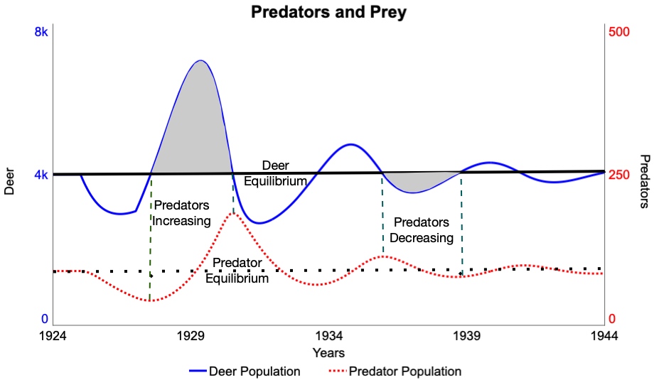
4.10.4. Building the Predator-Prey Model: Explanation of the Variables
The table below gives a detailed explanation of the variables in the predator-prey model in Figure 4.15 and specifies numeric values and ranges for variables. You will use this information to build the model in the next Action Item.
Explanation of the Variables int eh Predator-Prey Model in Figure 4.15, with Suggested Values Corresponding to the Mule Deer on the Kaibab in 1907
- Initial Deer Population: This is an exogenous variable that can be used to set (and change) the initial size of the Deer Population. Set this variable to be equal to 4000, with an input range running from 2000 to 8000 in increments of 100 deer (i.e. precision = 100) and set the scale = none.
- Deer Population, Deer Net Growth Rate, Baseline Fractional Deer Growth Rate, Actual Fractional Net Growth Rate, Kaibab Adequacy to Support the Deer Population, Ratio of the Deer Population to Carrying Capacity – See the discussion on the S-shaped growth model.
- Set the Deer Population to be equal to the variable Initial Deer Population.
- The Baseline Fractional Deer Growth Rate is 1.0 (meaning that there is, on average one deer born each year per each deer in the population). Set the input range to run from 0.1 to 1.5 in increments of 0.01.
- The Actual Fractional Net Growth Rate, Kaibab Adequacy to Support the Deer Population, and the Ratio of the Deer Population to Carrying Capacity variables are calculated the same way as in the original S-shaped growth model.
- Set the Kaibab Deer Carrying Capacity to be 40000, with an input range running from 4000 to 60000 deer in increments of 1000 deer.
- Deer Predation: The number of deer killed by predators each year. This is calculated as the product of the Baseline Annual Kills Per Predator, the number of animals in the Predator Population, and the Effect of Deer Density on Predator Efficiency (all explained below).
- Baseline Annual Kills Per Predator: The number of deer that would be killed per predator each year, assuming that there was a natural balance between the predator and deer populations. This variable is set to a value of 40 deer per predator per year (units are Deer/(Predators*Year)). Set the input range to run from 20 to 60 with the precision set to 1.
- Deer Density: A measure of how many deer there are in a given area on the Kaibab Plateau. This is measured as the number of deer per 1000 acres, and is calculated by dividing the Deer Population by the Kaibab Area in Thousands of Acres. This is then divided by the Normal Deer Density per Acre.
- Normal Deer Density per Acre: The number of deer per acre under ideal conditions. This value is set to 5 and has units of Deer/Thousands of Acres.
- Effect of Deer Density on Predator Efficiency: This is a dimensionless value used as a multiplier to increase or decrease the Deer Predation, according to the Deer Density level. This value varies between 0 and 1.5. Its value is 0 when there are no deer present (i.e. when deer density = 0 deer per 1000 acres) and it is 1.5 when there is an abundance of deer (i.e. when the deer density reaches 10 deer per 1000 acres or more). Hence, if there are no deer present, the Deer predation will fall to zero. If there is an overabundance of deer, the Deer Predation will be 1.5 times as great as it would be in equilibrium. This variable was formatted in the diagram to use a boldface, underline font to highlight that its value is not set by an equation, but by a graphical function showing how the Effect is calculated based on the Deer Density. That graphical (nonlinear) function is shown below.
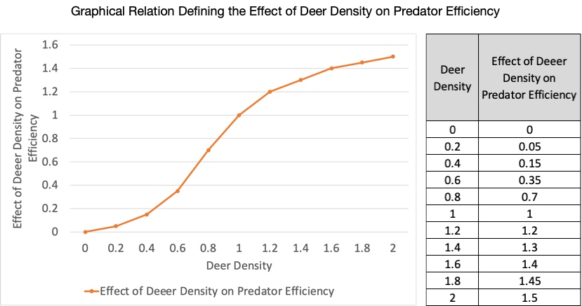
- Kaibab Area in Thousands of Acres: The size of the Kaibab Plateau; units are thousands of acres. Since the Kaibab plateau covers 800,000 acres, this variable is set to the value 800.
- Initial Predator Population: This specifies how many predators are in the ecosystem at the start of the simulation. Set this to be 90 predators. Set the input range to run from 20 to 130 in increments of 1 predator.
- Predator Population: The stock of predators in the ecosystem. Set the initial value to be equal to the variable Initial Predators Population.
- Net Predator Growth Rate: The net number of predators added to (or removed from) the Predator Population each year through the natural birth and death processes. This value is calculated as the product of the Predator Population, the Baseline Fractional Predator Growth Rate, and the Effect of Deer Density on Predator Births.
- Baseline Fractional Predator Growth Rate: This represents the fraction by which the Predator Population will grow each year, assuming there are an abundance of deer available for food. Set this value to 0.7 with an input range from 0.2 to 1.5 with a precision of 0.01.
- Effect of Deer Density on Predator Births: This is a dimensionless value used to represent how the Deer Density on the Kaibab Plateau affects the growth rates of the predator herd. This variable is used as a multiplier to increase or decrease the Net Predator Growth Rate, according to the Deer Density value (with greater density implying more food for predators, and hence a greater reproductive rate). This Effect of Deer Density on Predator Births variable is also determined by a graphical relationship with Deer Density. When the Deer density is 0, the Effect is -1.0, meaning that the Predator population will experience negative growth (from a lack of food). When the Deer density is 1, the effect is 0, meaning that the Predator Population will experience flat growth (neither growing nor shrinking). When the Deer Density is more than 2 , the Effect of Deer Density on Predator Births is 1.5, meaning that the Predator Population will grow at 1.5 times the Baseline Fractional Net Growth Rate (because there are abundant deer available for food). Below is the graphical function defining how the Effect of Deer Density on Predator Births is determined by the Deer Density.
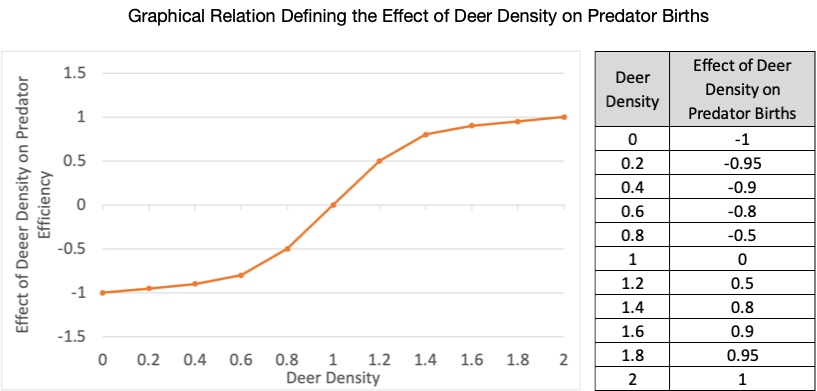
Exercises 4:16 Modeling Challenge – Build a Predator-Prey Model for the Kaibab Plateau
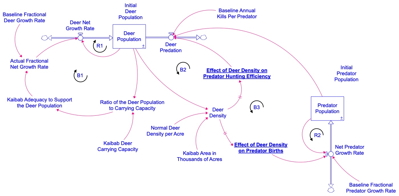
- Build the predator-prey model shown here.
- Use the following Model settings
- Start and end times: 1900 and 2000, respectively
- DT: 1/10 (note difference from earlier models)
- Time units: Years
- Integration method: RK4 (note: This is different than in previous models. We recommend that you use RK4 when dealing with oscillatory systems.)
- Make sure you …
- Fully document all units and variable descriptions
- Specify the input ranges for all exogenous variables, as specified in the above explanation of variables in the predator-prey model.
- Identify all of the variables and causal links involved in each feedback loop, so that Stella Architect® highlights the feedback loop when you place your cursor over the circular loop identifier.
- Get BOTGs that looks like the following two cases.
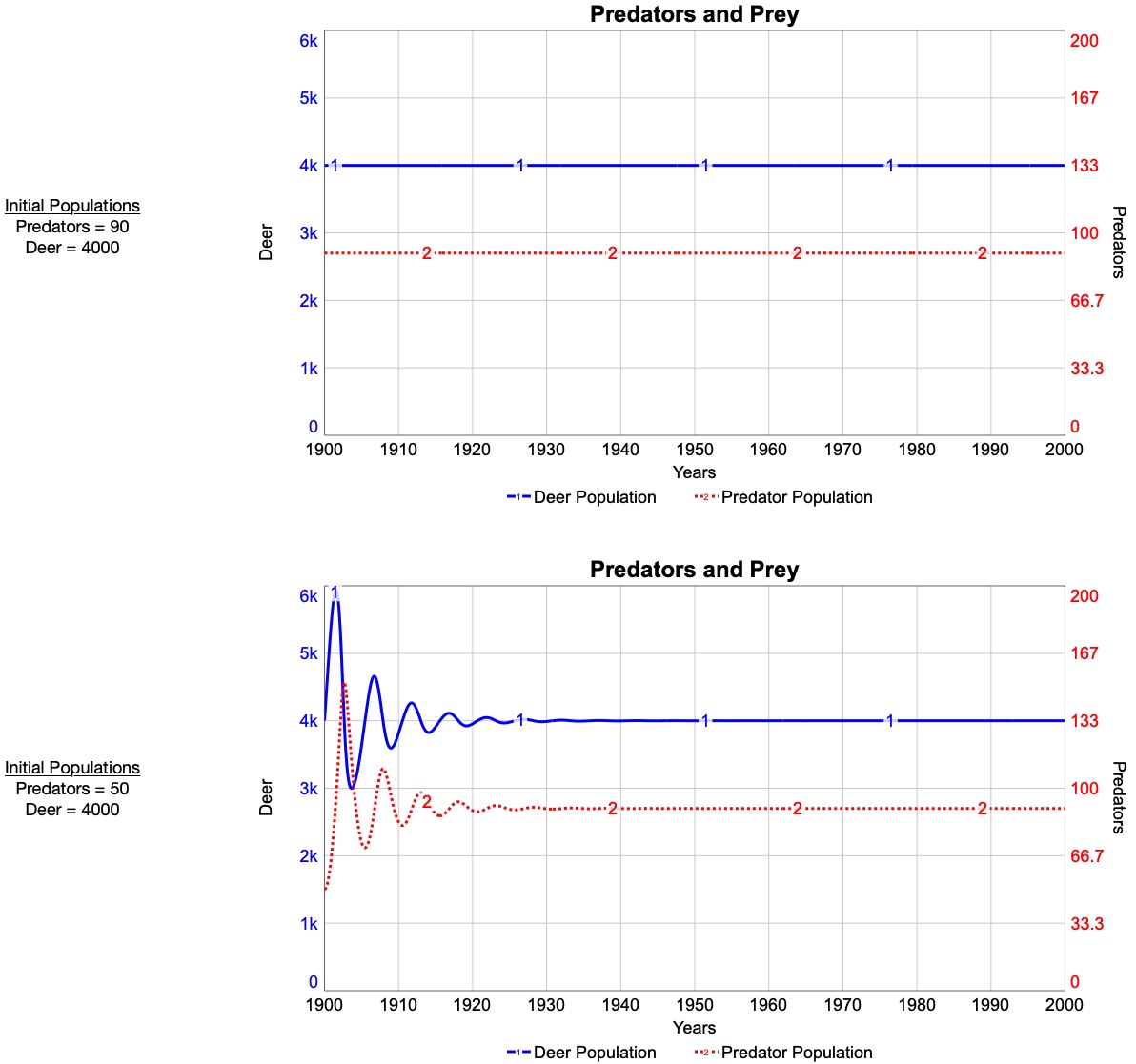
3. Create a user face with a main page like the one here and with a 3-page system story structured as you see below. You can also access an online version of the interface here to better view the details of what to include and how the interface works. The three pages in your system story should “unfold” the feedback structure in the system, as shown here.
You will create these pages and then add. your own text explaining how the feedback structure in the system works.
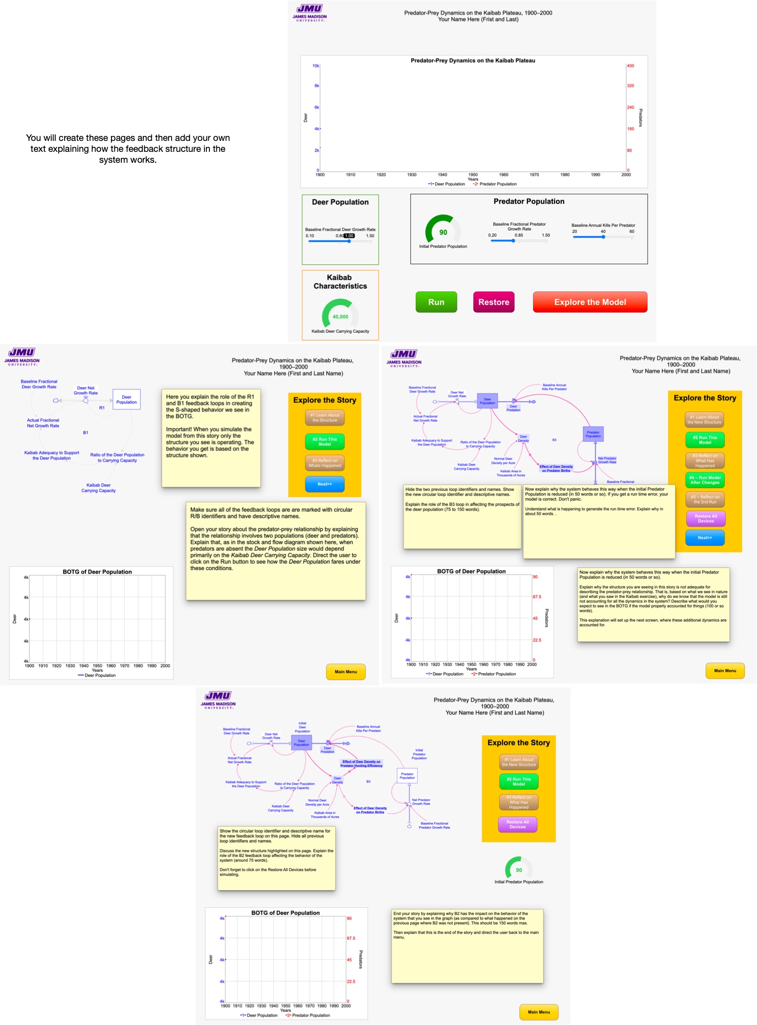
4. Now use your model interface to run some experiments on the model and to explore what effect each of the exogenous variables on your interface have on the behavior of the system.
-
- Overall, what seems to be the role of the Kaibab Deer Carrying Capacity in the behavior of the system? That is, when you change it, what happens? Why?
- Why don’t the deer oscillate around the carrying capacity value? What does this tell you about the role of the R1 and B1 loops in affecting the behavior of the system?
4.11. Putting it all Together: A Kaibab Ecosystem Model
4.11.1. You’ve Been Here Before
It’s now time to build model of the Kaibab ecosystem. This model will be very similar to the simulator you used in the Kaibab Challenge at the beginning of this Learning Guide. Creating this model will require you to combine many of the feedback structures you’ve already learned from previous models.
In the Kaibab Challenge, you were placed back in the early 1900’s and asked to make decisions so that the mule deer population on the Kaibab Plateau would grow and flourish for generations to come. You quickly discovered that this was no easy task. In fact, (just like those who actually worked on this problem in the early 20th century), you found that the most obvious approaches to growing the deer population (such as reducing the number of predators) would lead to disaster. In many ways, this unfortunate outcome was inevitable for the following reasons:
- You had misleading information: Many thought that the Kaibab could support up to 30,000-40,000 deer. Given that there were currently only 4000 deer on the Kaibab, it seemed obvious that measures could be taken to increase the population while remaining within the natural constraints of the ecosystem.
- Stakeholders muddied the decision making process: Your job was at stake! The President of the United States and your own boss had expectations that made it difficult for you to objectively choose the best course of action.
- The ecosystem behaved in counterintuitive (Forrester, 1971) ways: The deer population did not follow the trajectory you had hoped for while it seemed that all was going well, but then (for most of you) the deer population exploded and consumed all of the forage. When the forage disappeared, the deer population collapsed. For others of you, the deer population was on what looked like a promising growth trajectory, but you probably noticed that was still growing. This led to an uneasy feeling that the deer population might eventually grow to outstrip the capacity of the ecosystem.
By now you have learned that these challenges come from an underlying system with multiple competing feedback loops involving deer, predators, livestock, and the forest on the plateau. In the models you have built and explored, you’ve seen that even fairly simple systems can behave in ways that defy our common sense.
You now have practice with the tools of system dynamics to help you analyze problems involving feedback systems like the Kaibab Plateau. You can build simulators that explore how the important feedback dynamics in such systems affect their behavior over time. Armed with that kind of understanding, you are in much better position to make good decisions.
And so we return to the Kaibab Plateau and the mule deer population in the early 1900’s. Our purpose in doing so is to revisit the challenging problem armed with the tools of system dynamics and to see how simulating such a system can lead to better decisions in the future. You will produce a simulator and user interface, along with a system story to explain how the feedback structure in the system works to create the irruption and subsequent collapse of the Kaibab mule deer population when the predator population is reduced by too much. Your interface will allow the user to experiment with the system and find conditions which lead to a healthy, sustainable Kaibab ecosystem with a healthy balance between the deer, the predators, and the forest.
4.11.2. Building the Kaibab Ecosystem Model
Figure 4.19 shows the stock and flow diagram for the Kaibab ecosystem model, and exercise 17 provides a detailed description of all of the variables in the model, along with guidance on values, equations, units, and input ranges. Take a few moments to study Figure 4.19 and notice that this model is comprised from building blocks that correspond to the models from previous sections of this learning guide. These building blocks are:
- S-shaped growth. This structure is the basic building block for modeling the deer population. The carrying capacity in the model is determined by the ability of the Kaibab forest to generate enough forage to support the deer.
- A renewable resource that the population needs for survival. Because the deer population depends on the forage generated by the Kaibab forest, we augment the S-shaped growth structure by letting the carrying capacity be determined by the amount of forage in the forest. The amount of forage available is represented by the Forage Biomass stock in this part of the model. This stock is “drained” by an outflow representing the Forage Consumed by Deer. As the trees and plants on the Kaibab propagate and grow, this stock of biomass is replenished. This is represented by the inflow labeled Net Annual Forage Growth.
- Predator-prey dynamics. The predators are the wolves and cougars on the Kaibab. The prey are the mule deer. The same feedback structure is used here as in the original predator prey model.
In addition to these building blocks, the model in Figure 4.19 shows an additional outflow from the Predator Population to account for the removal of predators by hunting. In the early 1900’s it was believed that a reduction in the number of predators on the Kaibab would allow the deer population to grow from its current level of 4000 deer to higher levels. At the time, it was believed that the carrying capacity was somewhere between 30,000 and 40,000 deer. By allowing for predators to be removed by hunting, the model will let us evaluate the impact of that policy.
Following Figure 4.19, exercise 17 explains the physical meaning and role of each variable in the model. That table provides guidance that you can use to specify the units for each variable, along with the numeric values or equations used to calculate each variable, as appropriate.
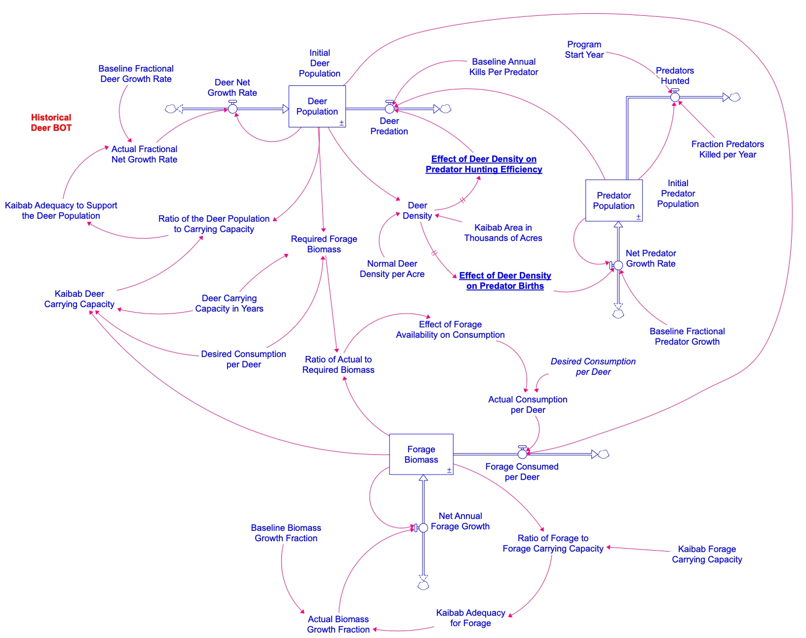
Exercise 17: Variable Description for the Kaibab Ecosystem Model |
||||
| Variables from the S-Shaped Growth Building Block, As Applied to the Kaibab Deer Population | ||||
| Variable | Physical Description | Numeric Value or Equation | Input Limits (for Interface) | Units |
| Deer Population | Left as exercise | Make equal to Initial Deer Population | Do not adjust | Left as exercise |
| Initial Deer Population | Left as exercise | 4000 | Do not adjust | Deer |
| Baseline Fractional Deer Growth Rate | Left as Exercise | 1.0 | 0.5 to 1.5 (precision = 0.01) | Left as exercise |
| Actual Fractional Net Growth Rate | Left as exercise | |||
| Kaibab Adequacy to Support the Deer Population | Left as exercise | |||
| Ratio of the Deer Population to Carrying Capacity | Left as exercise | |||
| Kaibab Deer Carrying Capacity | Left as exercise | Forage Biomass/(Desired Consumption per Deer*Deer Carrying Capacity in Years) | Nothing to adjust | Left as exercise |
| Variables from the S-Shaped Growth Building Blocks, as Applied to the Forage Biomass on the Kaibab | ||||
| Variable | Physical Description | Numeric Value or Equation | Input Limits (for Interface) | Units |
| Forage Biomass | Forage available for deer to eat | Initial Value = 317000 | Do not adjust | Metric Tons |
| Baseline Biomass Growth Fraction | Left to exercise | 0.10 | 0.05 to 0.25 (precision = 0.01) | Left as exercise |
| Actual Biomass Growth Fraction | Left as exercise | Left as exercise | Do not adjust | Left as exercise |
| Net Annual Forage Growth | Net change in the forage biomass on the Kaibab via natural growth and decay, apart from consumption by animals. | Left as exercise | Do not adjust | Left as exercise |
| Kaibab Adequacy for Forage | Left as exercise | Left as exercise | Do not adjust | Left as exercise |
| Ratio of Forage to Forage Carrying Capacity | Left as exercise | Left as exercise | Do not adjust | Left as exercise |
| Kaibab Forage Carrying Capacity | Amount of forage biomass that the Kaibab can support on an ongoing basis. | 350000 | 200000 to 600000 (precision = 1000) | Left as exercise |
| Forage Consumed per Deer | Left as exercise | Left as exercise | Do not adjust | Left as exercise |
| Variables dictating the interdependence between the deer population on the forage ( a renewable resource). Use the model from section 4.10 as a building block for this section. Things make look slightly different, but the concepts should hold. | ||||
| Variable | Physical Description | Numeric Value or Equation | Input Limits (for Interface) | Units |
| Actual Consumption per Deer | Left as exercise | Left as exercise | Left as exercise | Left as exercise |
| Desired Consumption per Deer | The amount of forage consumed by a single deer in a year, when abundant forage is available. | 0.75 | 0.4 to 0.8 (precision 0.01) | Left as exercise |
| Ratio of Actual to Required Biomass | Measures how much forage is available, relative to what is need to sustain the current deer population. Values below 1 indicate a shortage of forge biomass. | |||
| Effect of Forage Availability on Consumption | This nonlinear or graphical function captures how Actual Consumption per Deer will change given the Ratio of Actual to Required Biomass. Deer will continue to eat a normal amount of forage until only about 30 percent of what is need is available. Deer will then start to eat less as foraging becomes more difficult. | 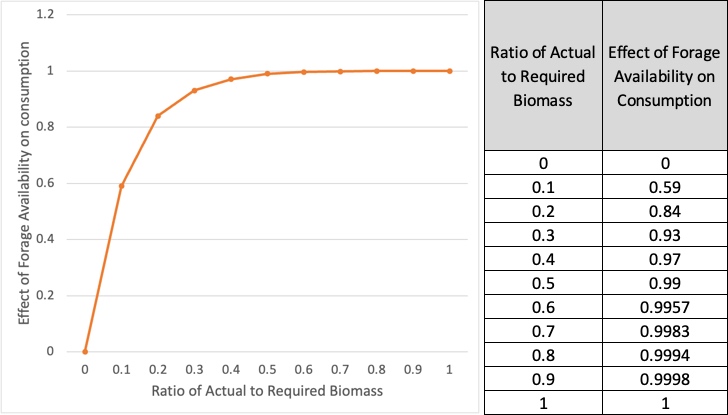 |
Dimensionless | |
| Deer Carrying Capacity in Years | Number of years of forage needed to sustain the deer population. | 2 | 1 to 7 (precision = .1) | Left as exercise |
| Required Forage Biomass | Forage biomass needed to sustain the existing deer population for the number of years indicated by the value of the Deer Carrying Capacity in Years. | Left as exercise | Left as exercise | Left as exercise |
| Variable from the Predator-Prey building block (as applied to the deer and predators on the Kaibab). | ||||
| Variable | Physical Description | Numeric Value or Equation | Input Limits (for Interface) | Units |
| Predator Population | Number of predators on the Kaibab Plateau | Initial Value = Initial Predator Population | Do not adjust | Predators |
| Initial Predator Population | Used to set the initial size of the Predator Population. Notice that this is different from the original predator-prey model you built. | 100 | Provided above | Predators |
| Net Predator Growth Rate | Left as exercise | Left as exercise | Do not adjust | Left as exercise |
| Baseline Fractional Predator Growth | Left as exercise | .5 | .5 to 1.5 (precision = 0.01) | Left as exercise |
| Effect of Deer Density on Predator Births | See the
Explanation of the Variables in the Predator-Prey Model in Figure 29, with Suggested Values Corresponding to the Mule Deer on the Kaibab in 1907 |
Left as exercise | ||
| Effect of Deer Density on Predator Hunting Efficiency | See the
Explanation of the Variables in the Predator-Prey Model in Figure 29, with Suggested Values Corresponding to the Mule Deer on the Kaibab in 1907 |
Left as exercise | ||
| Deer Density | The ratio of deer to area all of which is divided by a normal. Results in a scale where one is normal and anything above 1 indicates that you have too many deer and anything below one indicates that you have to few deer compared to what is normal deer per acres. | Deer Population / Kaibab Area in Thousands of Acres / Normal Deer Density per Acre | Do not adjust | Left as exercise |
| Kaibab Area in Thousands of Acres | Land area of the Kaibab Plateau. This is approximately 800,000 acres. We are measuring this in thousands of acres so that is why we use 800 when setting the value. | 800 | Do not adjust | Left as exercise |
| Normal Deer Density per Acre | Number of deer per 1000 acres on the Kaibab | 5 | Do not adjust | Deer/Thousands of Acres |
| Deer Predation | Left as exercise | Left as exercise | Left as exercise | Left as exercise |
| Baseline Annual Kills per Predator | The average number of deer killed per predator in a given year. | 40 | 20 to 60 (precision = 0.1) | Deer/(Predator*Years) |
| Variables related to the predator removal by hunting. | ||||
| Variable | Physical Description | Numeric Value or Equation | Input Limits (for Interface) | Units |
| Predators Hunted | Number of predators removed each year through hunting.
The STEP is a built in function. The operation in the parentheses will not occur until the Program Start Year is reached. Make sure you include the comma as this separates |
Step(Predator Population * Fraction of Predators Killed per Year, Program Start Year) | None | Left as exercise |
| Fraction Predators Killed per Year | Fraction of predators killed each year. | 0 | 0 to .5 (precision = .01) | Left as exercise |
| Program Start Year | The year the predator hunting policy is implemented. From that year on, a fraction of the remaining predators will be hunted and killed each year. | 1907 | 1905 to 1920 (precision = 1) | Left as exercise |
| Other Ancillary Variables | ||||
| Variable | Physical Description | Numeric Value or Equation | Input Limits (for Interface) | Units |
| Historical Deer Behavior Over Time Graph | A reference mode showing the actual deer population estimates from 1900 through 1950. This is defined by the graphical function shown here. You can display this BOTG with the Deer Population to help us tune the model parameters to match the historical record. | 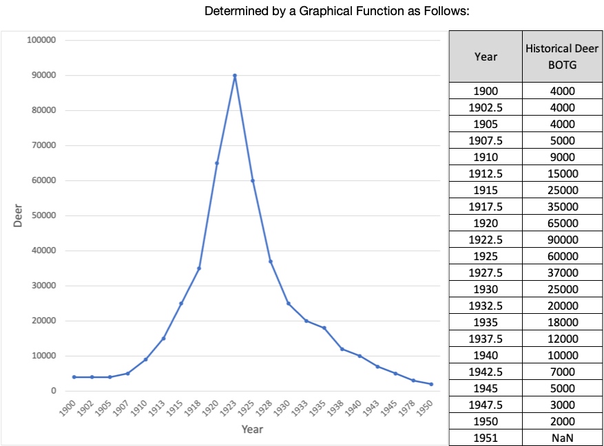 |
Deer | |
Exercises 4:18 Modeling Challenge – Build Kaibab Model and User Interface

- Build the Kaibab ecosystem model shown here. Use the descriptions of the variables in Exhibit 4.11 to guide your efforts. As you build the model, pay attention to the following:
- Document the physical meanings and units of every variable
- Label the polarities of all causal links using the +/- notation.
- Identify all feedback loops and label/number the loops with the circular identifiers and numbered labels (R1, R2, B1, etc)
- Make sure that all the links and variables involved in a given feedback loop are highlighted whenever you pass your cursor over the circular loop identifier.
- Use the following model settings
- Start time: 1900
- Stop time: 1950
- DT = 1/20 year
- Integration method: RK2
- Time units: years
- Check your model to make sure it is running correctly by making sure you get the following BOTGs.
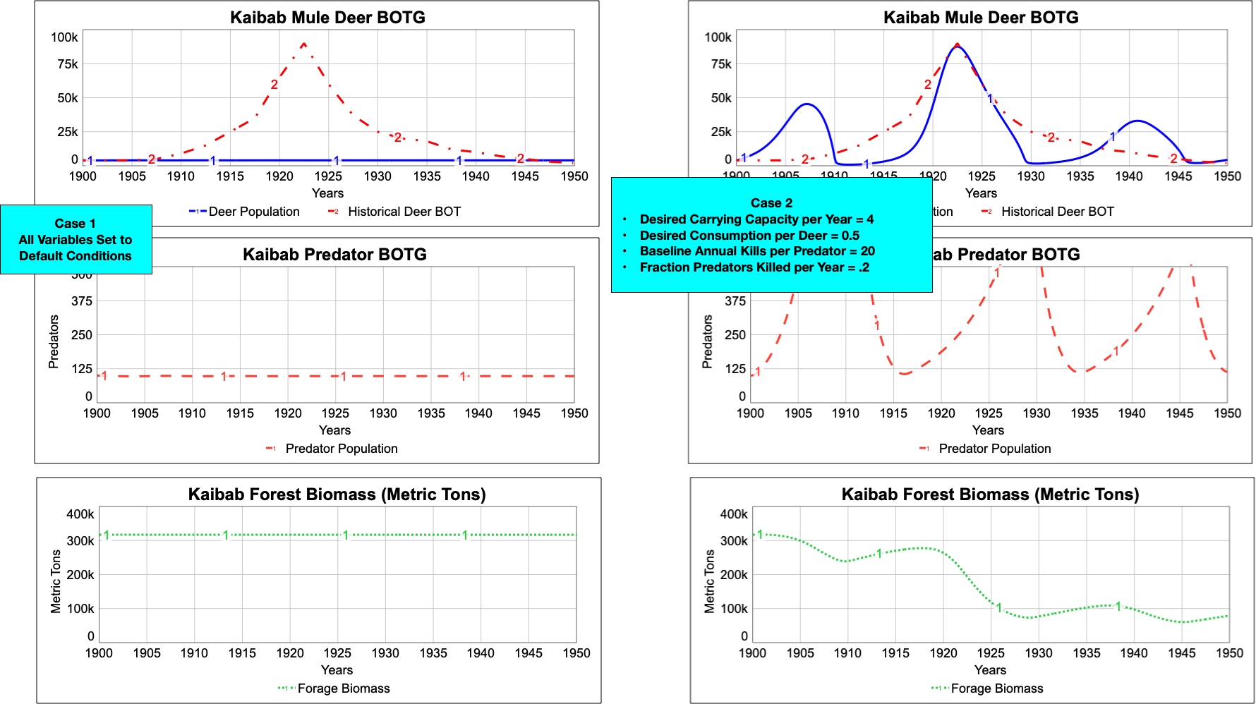
3. Build a user interface to match this online working version and also shown below.
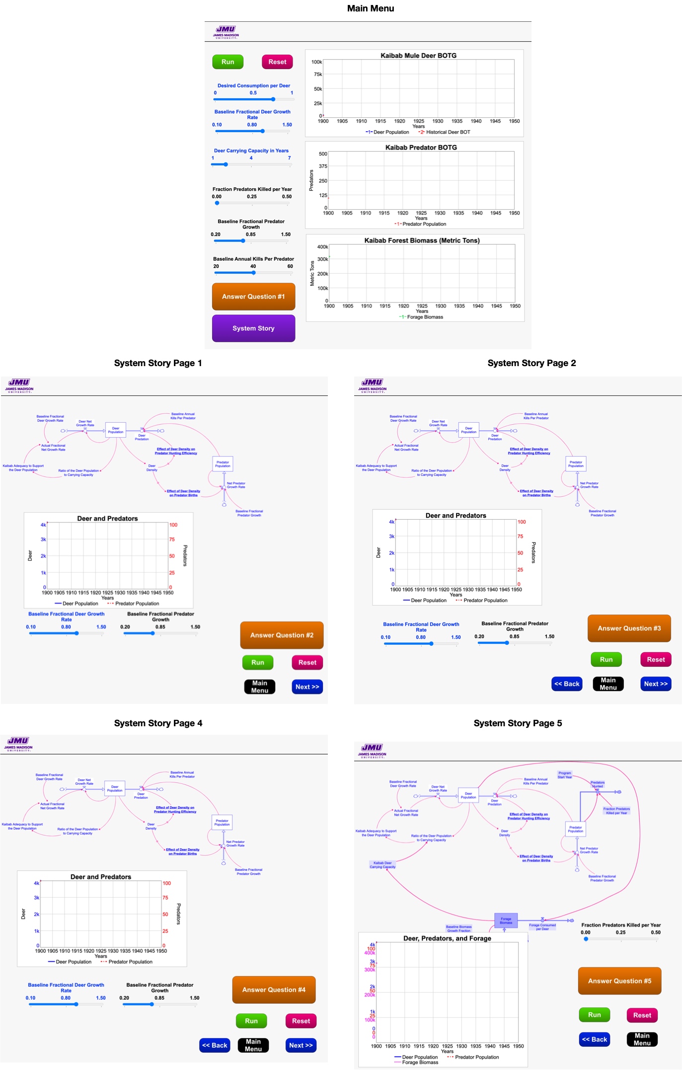
4. Adjust the model parameters to match as closely as you can the historical BOTG. As you do this, make sure that your adjustments have some connection to reality by keeping in mind the following facts:
-
- Somewhere between 800 and 1500 predators were removed via hunting from 1907 through 1932.
- The annual net growth fraction for deer is somewhere between 0.7/years and 1.2/years.
- The annual net growth fraction for the predators is somewhere between 0.5/years and 1.2/years.
- In the 1920’s the Kaibab forest started showing signs of severe overconsumption from the deer population.
- You can get a dampened oscillation if you insert a delay in the balancing feedback loop. You should also note that all software packages have built in formulations that allow you to easily add delays, but you are hiding the stock and flow structure. ↵
- See Sterman (ibid), page 34 for a brief discussion of the history of these terms. ↵
- See Deaton and Winebrake (2000). Dynamic Modeling of Environmental Systems, Springer-Verlag and Ford (2009). Modeling the Environment, 2ed. Island Press. ↵
The order of a system is determined by the number of stocks in a feedback loop. A feedback loop with two stocks would be a second order system while one with five feedback loops would be a fifth order system.


Feedback/Errata